
Disk Detective–in Chinese!
We’re excited to announce that Disk Detective has been translated into Mandarin Chinese–both simplified and traditional character fonts! Many thanks to Ruobing Dong at the University of California, Berkeley Astronomy Department and Mei-Yin Chou at Academia Sinica’s Institute of Astronomy & Astrophysics (ASIAA) for the translation work and to Chris Snyder at Zooniverse for the technical work.
Here is a brief description of Disk Detective in traditional character Chinese and then followed in English:
類似地球的行星是在圍繞著年輕恆星的氣體、塵埃、岩石和冰塊所構成的盤中形成。我們需要你的幫忙來找出更多這種孕育行星的盤,這樣我們才能找 到系外行星且更加了解它們如何成長。
為了找到這些盤,我們結合了數十萬張來自美國太空總署(NASA)的廣域紅外線巡天探測(WISE)任務的影像。已經有很多科學家搜尋來自 WISE的資料並試著用電腦找出這些盤。然而這些盤容易跟星系、小行星、星際物質團塊和其他天體搞混,科學團隊檢視後發現必須用人眼來辨識這 些資料才行。
在尋盤偵探(DiskDetective.org) 中,有了你的協助,這些被辨識出來的盤將能用來建立一個最大的盤資料目錄。NASA的James Webb太空望遠鏡和其他望遠鏡將用這個目錄為主要目標來尋找系外行星。我們找到的這些盤將有助於了解太陽系的過去跟未來。
http://www.diskdetective.org/?lang=zh_tw
Planets like the Earth form within disks of gas, dust, rock and ice grains that surround young stars. We need your help to find more examples of these planet-forming disks so we can locate extrasolar planets and better understand how they grow and mature.
To find these disks, we’re combing through a catalog of hundreds of thousands of sources from NASA’s Wide-field Infrared Survey Explorer (WISE) mission. Many scientists have been searching through the data from the WISE space telescope to find disks using computers. But the disks are mixed in among galaxies, asteroids, clumps of interstellar matter, and other contaminants. And each team that has looked through the data has found that every source has to be verified by eye.
With your help, at Disk Detective.org we will produce a catalog of verified sources many times bigger than any other catalog. This catalog will yield key targets for NASA’s James Webb Space Telescope and other telescopes to search for exoplanets. The disks we find will help us understand the history and future of our solar system.
Good News Everyone! 272,000 More Subjects
January 28 we launched DiskDetective with a first batch of about 32,000 sources to classify. Of these, 20,000 have been in rotation at any given time. That’s a lot of astronomical data–and a lot of flipbooks to look at.

Well, it completely shocked us when we heard in March that some folks were seeing repeats–meaning that they had already classified more than 20,000 subjects! Now, we had always planned to have many more subjects than that in Disk Detective. But at that point, we were still in the process of downloading the data from the NASA/IPAC Infrared Science Archive onto a hard drive on Marc’s living room carpet, a process that took about a month. So we weren’t ready to put any more data online to keep all our detectives detecting.
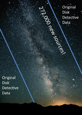
The figure below shows the distribution of the J magnitudes of the sources with excess emission at 22 microns that WISE made really high quality images of (specifically ones from Southern Galactic latitudes, but that doesn’t matter). The total distribution, shown by the black curve, has two peaks, one around J=9, the other around J=16.
What is the meaning of these two peaks? Could it be two different kinds of sources?
The red and orange curves tell the rest of the story. The red curve shows the numbers for just those sources close to the Galactic plane. The orange curve shows the numbers for the remainder of the sources–those far from the galactic plane. Dividing the sources up in this manner shows that the second peak is mostly due to distant galaxies.
At low galactic latitude, dust from our Galaxy, the Milky Way, obscures most galaxies external to our own. So we know that the objects shown by the red curve–most of the peak at J=9–are stars (and maybe stars with disks). At high galactic latitude, the opposite is true. The objects shown by the orange curve should be mostly galaxies. That’s the peak at J=16.
For now, we’d like to skip the objects that are mostly galaxies (orange curve) and concentrate on the objects that are mostly stars (red curve). The orange and red curves cross at about J=14.5, so we decided to put aside the objects with J > 14.5 for now. That means this new batch of data should have fewer galaxies in it than the old batch–and more of those delicious disks!

What are we doing with the sources with J magnitude >14.5? Don’t worry, we’ll be putting them to good use. Our colleagues have suggested that hidden among those fainter sources could be Kardashev Type II and Type III civilizations. So once we’re done with this new batch of sources (roughly in 2017), we’ll start looking at the fainter objects–looking for signs of extraterrestrial intelligence. In fact–you may have already spotted some in the first batch of data. (They look just like debris disks and very red galaxies). Stay tuned!
Follow-Up Observing Begins!
In our last blog post, we invited you to submit interesting targets to follow up with the Tillinghast 1.5m telescope at Mt. Hopkins this spring. Thank you to jessicamh, Gez Quiruga, arvintan, kmasterdo, silviug, wtaskew, cpitney, Pini2013, Ted91, Vinokurov, michiharu and everyone else who submitted targets! Thanks to your help, we picked out 102 objects to follow up this spring. The observing starts tomorrow night.
And guess what? We’ve got more follow-up observing planned for the fall semester, and also for the Southern hemisphere, with help from our new collaborators, Luciano Garcia and Mercedes Gomez from Observatorio Astronómico de Córdoba and Christoph Baranec from the University of Hawaii.
So we’re keeping that target submission form open. From now on, whenever you find an interesting target, anywhere in the sky, feel free to submit it.
And now that we’ve been through this process, I can better explain how we decided what to follow up this time. This part of the blog post is going to be a bit technical–so feel free to skip it, or ask us for more info if you get tripped up by the jargon.
We started by searching SIMBAD and VizieR for information on each object, keeping the search radius to 0.2 arcminutes. These are the kinds of objects we most want to follow up:
Main sequence stars (aka dwarfs)
Luminosity Class IV stars: A IV, F IV, G IV, K IV, M IV.
A III, F III, G III and K III stars
T Tauri stars and Herbig Ae stars
white dwarfs
objects with distance < 200 parsecs
objects with proper motion > 30 milliarcsec/year
shell stars
We generally don’t want to follow up:
M giants
Cepheids
Be stars
galaxies, Active Galactic Nuclei
blends (i.e. two objects so close together that we can’t analyze them separately)
eclipsing binaries
O stars
supergiants
Also mixed in the lists of possible targets were:
binary stars
known disks
and plenty of objects where we can’t tell what it is
These objects went onto a “Maybe” list, to be followed-up as second priorities.
We could read some of this information from the SIMBAD spectral type. The quality of this information varies, and the SIMBAD spectral type includes a data quality letter (A,B,C,D, or E) where A is the best. Since the purpose of this observing run is to weed out blends and to get more accurate spectral types, we figured it was OK to look at objects where the spectral type quality was poor. But we threw out objects classified in SIMBAD or VizieR as M giants, Cepheids, Be stars, galaxies, Active Galactic Nuclei, eclipsing binaries, O stars or supergiants.
The most common contaminants are M giants and supergiants. We want to avoid those. But some M stars are main sequence stars (dwarfs). Like this one: AWI00003dm Disks around these M dwarfs are rare and interesting and worth extra points! So we must be careful weeding out the M giants and supergiants.
M giants are sneaky! They come with many different labels in SIMBAD and VizieR: Long Period Variables (LPVs), SR+L, Slow Irregular Variables, Miras, Semi-regular Variables, Semiregular pulsating Variables, Carbon stars. All those are kinds of M giants/supergiants and they tend to make their own dust, so we can’t use dust around them as an indicator of a planetary system. We’re not following them up.

M dwarf disks are exciting but rare. Here’s a Hubble picture of one around a star called AU Microscopii.
Sometimes you can spot an M giant even when there’s no known spectral type. For example, subtract the V magnitude from the K magnitude. If V – K > 3.29, you’re looking at an M star. Then, if a star has a measured distance of thousands of parsecs, you can bet it’s a giant or supergiant. So we declared some objects to be M giants based on color and distance. A real M dwarf is so faint we can only see it if is much closer than 100 parsecs.
Here’s more information about how to guess a star’s spectral type based on its color: http://www.stsci.edu/~inr/intrins.html
If you know you’re looking at an M star, another good clue that it’s a giant/supergiant is if it is highly variable (e.g. amplitude more than one magnitude). So we looked up the variability amplitude for our targets in VizieR as well.
For an M star with no parallax measurement and no variability measurement, it can be hard to tell if you’re looking at a dwarf of giant or supergiant. So I put objects like that on the “maybe” list.
And finally–all the subjects on Disk Detective are preselected to have a certain degree of redness (we require the WISE 4 magnitude to be at most the WISE 1 magnitude – 0.25). But that’s not sufficient to find M star debris disks, since M stars are so cold, and therefore intrinsically red colored. We had to additionally weed out M stars with WISE 4 magnitude > WISE 1 magnitude + 1.0. (I know that sounds terribly confusing–it’s confusing because in the astronomical magnitude system, brighter objects have lower magnitudes. But adding this second criterion says that we are being more demanding when it comes to M stars in terms of how much brighter they need to be in the WISE 4 band than the WISE 1 band.)
Whew—that’s a lot of detail, I know. But now you can see why we try to weed out all those blends and multiples etc. using the handy animated flipbooks on the DiskDetective site before we start all the detailed research on each one.
Here are all the objects on our current version of the follow-up list for the Tillinghast 1.5 m for this spring, below (this list includes the maybes). Thanks again for all your hard work. And keep our fingers crossed for good weather at Mt. Hopkins!
Marc
| Zooniverse ID |
| AWI0000bs0 |
| AWI0000tjx |
| AWI0000gjb |
| AWI0000fye |
| AWI0000kg4 |
| AWI0000ojv |
| AWI0000tz1 |
| AWI0000u8s |
| AWI0000uj2 |
| AWI0000uji |
| AWI0000w9x |
| AWI0000ibq |
| AWI0000v1z |
| AWI00006nk |
| AWI00000wz |
| AWI0000tgc |
| AWI00002ms |
| AWI0000cot |
| AWI0000nwt |
| AWI00002zo |
| AWI0000m2p |
| AWI0000ns8 |
| AWI00004o8 |
| AWI000050r |
| AWI0000hjr |
| AWI000048c |
| AWI00005uf |
| AWI00000o6 |
| AWI00001l8 |
| AWI00002yt |
| AWI0000hog |
| AWI0000kk6 |
| AWI0000eg6 |
| AWI000004g |
| AWI00007qu |
| AWI000001j |
| AWI00001q1 |
| AWI00005xz |
| AWI00006bt |
| AWI00004qc |
| AWI00000zp |
| AWI0000kgo |
| AWI00007dp |
| AWI00000om |
| AWI00006dp |
| AWI0000149 |
| AWI000011b |
| AWI0000l8w |
| AWI0000us7 |
| AWI0000gz9 |
| AWI000028h |
| AWI0000vk9 |
| AWI0000jo8 |
| AWI000015r |
| AWI00000au |
| AWI000066t |
| AWI00002xh |
| AWI00006kc |
| AWI0000632 |
| AWI0000np1 |
| AWI00002fw |
| AWI00006p0 |
| AWI0000ajw |
| AWI00007i1 |
| AWI000047d |
| AWI0000tpu |
| AWI0000qxd |
| AWI0000hat |
| AWI000055c |
| AWI0000wip |
| AWI00006b3 |
| AWI0000tsh |
| AWI00002hx |
| AWI000054k |
| AWI00001sw |
| AWI0000r07 |
| AWI0000t35 |
| AWI0000a7e |
| AWI000019z |
| AWI0000s7e |
| AWI0000wqx |
| AWI00005x2 |
| AWI000042e |
| AWI0000aoe |
| AWI00004ox |
| AWI00000lj |
| AWI00000my |
| AWI000034n |
| AWI00004c1 |
| AWI00005ko |
| AWI00006hl |
| AWI00006nb |
| AWI00007fu |
| AWI00007ne |
| AWI0000c02 |
| AWI0000l70 |
| AWI0000s8t |
| AWI00006m2 |
| AWI000072k |
| AWI0000qnj |
| AWI000016c |
Send Your Favorite Targets!
Detectives,
You may recall that in February, we submitted our first follow-up observing proposal. We asked for two nights of time on the FAST spectrograph on the Tillinghast 1.5m telescope at the Fred Lawrence Whipple Observatory.
Well, not only did the time allocation committee like our proposal. They gave us more time than we asked for! Depending on the weather, it looks like we will have about four nights to follow up our favorite good candidates.
So now we need to make a new list of targets, and we need your help!
Please send in your suggestions using this online form. We’re looking for objects that are:
1) Good candidates in Disk Detective.
2) Mostly in the Northern hemisphere. So make sure the declination is > -20 degrees.
3) Up at night during the months of May-July. That means the Right Ascension of the object should be less than 25 degrees, or greater than 120 degrees.
4) Bright enough to see with this telescope. That means V magnitude < 15. You can find the V magnitude for some of the objects at SIMBAD through the Talk pages. For other objects, you have to look in VizieR. Remember, when you search VizieR, change the search radius to 0.2 arcminutes, to match the WISE beam at 22 microns.
5) And while you’re looking in SIMBAD and VizieR, jot down the spectral type, parallax, the J magnitude, the proper motion, etc.
On this observing run, we will be collecting medium-resolution spectra of the targets, to check if they are indeed stars, and to get better measurements of their luminosity classes–whether they are on the main sequence or not. So if there is not much information in the literature about the spectral type, that’s OK.
But some targets will be clearly identified as giants, or supergiants, or Cepheids, Miras, Be stars, RR Lyrae stars, or Long Period Variables. These kinds of stars all make their own dust, so finding a disk around them doesn’t indicate a planetary system. You can send those in if you want, but they won’t be our first priority this round. For now, we’re mainly interested in dwarfs and subgiants (luminosity classes IV and V) and even white dwarfs, if you can find them.
Send in your new target suggestions–as many as you like–in by this Friday (April 11). And if you can’t find any in time this week, don’t worry! We’ll be applying for more observing time later on.
Here’s the URL for that submission form: https://docs.google.com/forms/d/1DfmYSrg614osuLaUsac_a03dX-Bt6Ab2ep5SXC4XWHw/viewform
Good luck!
Best,
Marc
Chasing Dust Around Dead Stars
The typical place to find dusty debris disks is orbiting around ordinary stars like the Sun, or younger stars that are in the process of forming terrestrial planets. But some dusty disks that you might spot in Disk Detective surround tiny, exotic dead stars called white dwarfs.

An artist’s impression of the evolution of a planetary system from middle-age to the star’s eventual death as a white dwarf. In the process, surviving asteroids can form a dusty disk around the white dwarf. Credit: Mike Garlick
Most ordinary stars like the Sun will end their lives by bloating up into red giants. The cores of the red giant stars are balls of mostly carbon and oxygen, the spent fuel of the nuclear burning that powers the star. Red giant stars blow away much of their mass in winds, and eventually become stripped down to naked cores. It is called a white dwarf when those winds are done blowing, and there is nothing left of the star but its carbon and oxygen core covered with a very thin layer of hydrogen gas. White dwarfs are just a bit larger than the Earth in diameter, though they generally weigh around three-quarters as much as the Sun!
For a long time people thought that the process of stellar evolution into white dwarfs meant certain death for any planetary systems that might orbit the original stars. Indeed, inner terrestrial planets may indeed be destroyed by this process. But large asteroids, giant planets, and potentially even icy bodies might survive if they are big enough and far enough away to weather the drastic changes that a star goes through. Astronomers are now studying the nearest white dwarfs for signatures of these possible surviving planets.
One telltale signature is the presence of dust orbiting a white dwarf. If we look at a white dwarf in infrared light, with a telescope like the WISE telescope, a dusty white dwarf will be brighter there than at shorter wavelengths, just like the targets of Disk Detective. Thanks to many observations of white dwarfs with the Spitzer Space Telescope, WISE, and NASA’s ground-based Infrared Telescope Facility, we have discovered a few dozen dusty white dwarfs in the last 10 years. We believe the dust around these stellar ghosts comes from asteroids kicked too close to the central white dwarf by a larger planet. When this happens, the asteroid shreds apart much like Comet Shoemaker-Levy 9 did when it collided with Jupiter in 1994, and the pieces of it form a disk around the white dwarf. The size of the disk is not much larger than Saturn’s rings.
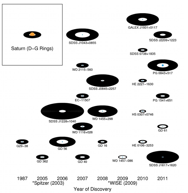
A collection of nearby white dwarfs and their accompanying dust disks. The dust disks are drawn to scale with Saturn’s rings. Credit: John Debes
Dust from the disk continues to rain down on the white dwarf surface in the form of atomic gas. Astronomers can measure the composition of this atomic gas—and thereby that of the dust—by taking optical and ultraviolet spectra of the white dwarfs. Just like characters from TV shows like CSI break materials found in a crime scene down to their component elements to identify them, astronomers compare the pattern of elements to Solar System bodies to understand the origin of the dust. Sure enough, they look just like asteroids in our own Solar System.
By chasing this elusive dust around dead stars, astronomers are using these clues to piece together the chemical history of terrestrial planet formation around other stars using the shredded remnants of exo-asteroids. The information they gain from studying white dwarfs might be able to tell us whether terrestrial planets have similar properties to our own Earth.
John Debes
Our First Follow-Up Observing Proposal
Barely a week after the launch of DiskDetective, I looked at the calendar and saw an important deadline looming: the deadline to propose for time on the telescopes at the Fred Lawrence Whipple Observatory (FLWO). The FLWO is a cluster of telescopes nestled into the rocky terrain at the peak of Mount Hopkins, about an hour south of Tucson, Arizona. Among this group of telescopes is the 1.5m Tillinghast, which our science team members Thayne Currie and Scott Kenyon have used in the past for spectral typing large sample of stars—the perfect machine for some initial follow up of our Disk Detective candidates.

The telescopes are scheduled by trimester, so there are opportunities to propose once every four months. But filled with excitement from our launch, and all the interesting candidates you have been discussing up on Talk, I was suddenly eager to jump on this chance to take our disk search to the next level. So I emailed the science team and we all started writing.
Proposing for time on a telescope generally means preparing a four to six page document (the proposal) and submitting it to the Time Allocation Committee (TAC). The TAC, a panel of astronomers who have experience using the telescope at hand, compares all the proposals the receive and decides how many nights on the telescope to award each one. The telescopes are always oversubscribed, so the TAC generally has to disappoint many of the teams that propose, awarding them fewer nights than they ask for, or maybe none at all.
In any given proposal round, the Hubble Space Telescope is usually oversubscribed by a factor of four to one. The brand new ALMA telescope was recently oversubscribed by a factor of nine to one! But the 1.5m TiIllinghast is only oversubscribed by about 1.5 to one, so it seemed like there is a good chance we will get some observing time to test our ideas, if we could somehow get our act together in a flash.
The proposals generally consist of a list of targets, a description of the observing procedure and how the data will be analyzed, and a few pages explaining why the work is important (the “Science Justification”). Each section must be perfect if it is going to impress the TAC. With only three days to go, John Debes and I started passing around a draft of the science justification section. Thayne Currie and Scott Kenyon chimed in on the observing procedure and data analysis sections.
The concept of the proposal was simple. Many of the good candidates from Disk Detective (clean, uncontaminated point sources whose spectra energy distributions look like a star plus a disk) are stars that we know very little about. We may know how bright they are in one or two bands, or even have a crude spectrum. But for a disk candidate to be useful to help us understand how, where, and when planets form, we need to know more than that.
We need to know whether the star is on the main sequence like the Sun, whether it as a young star like HH 30, or whether it has evolved off the main sequence, like the red supergiant Betelgeuse. We need to know the star’s mass—stars range in mass down to less than one tenth of the Sun’s mass, and up to maybe 100 times the Sun’s mass. And of course, we need to be certain that the object we think is as star is not really a galaxy or AGN. The observations we had in mind can help fill in all this information by telling us the “spectral type” of the star.
The 1.5m Tillinghast telescope (the 1.5 meters refers to the diameter of the first mirror that the starlight hits) comes with your choice of two different spectrographs. We opted to propose for the FAST spectrograph, which provides spectra with a moderate level of resolution, but has a very high efficiency, so we will have time to take spectra of maybe 50 stars per night. If you’re used to looking at the SEDs of your favorite object, you can think of these spectra as filling in some of the fine details in the SEDs in the wavelength range around 0.4 to 0.7 microns. The fine details will show us absorption lines (dips in the spectrum) associated with various elements in the star near its surface. The widths of the lines tell us about the star’s mass. The relative strengths of the different lines will tell us the star’s temperature. With a bit of additional modeling, we can also learn about the amount of each element present in the star and even constrain the star’s age.
So the concept was straightforward, as far as these things go—business as usual for astronomers who study stars. What was scary about writing this proposal was the target list! We didn’t need to make the final selections just yet; if we win the telescope time, we will be allowed to submit the final list later on. But at this point we had to understand going in what kinds of targets were available if we were going to write something reasonable. Alissa Bans started digging through the data from the Disk Detective classifications and quickly got stuck; there was already just too much data from the more than 250,000 classifications we had already received to sort through and comprehend in one weekend. I thought for a bit that we were going to have to give up, and wait till next round.
Fortunately, at the same time, the Disk Detectives were submitting their favorite objects on the Talk pages, checking the RA and Dec in SIMBAD to make sure they were in the right part of the sky for this telescope to observe in the spring trimester, checking the V magnitude to make sure collecting a high quality spectrum wouldn’t take too long, and checking the literature to make sure they had not already been classified. In about 24 hours, we had lists of good targets from Pini2013, TED91, onetimegolfer, artman40, silviug, WizardHowl, Vinokurov and others. These lists gave us a notion of how our target options were distributed in terms of observability and what was known about them. And the mere fact that y’all were able to come up with these lists of good targets made us confident that the proposal was worth submitting, even in such a rush.
Tuesday morning, Scott Kenyon uploaded the finished proposal onto the proposal submission website. In a few weeks, the TAC will make its decision. With any luck we’ll be awarded a night or two of time to start following up our objects.
If that happens, none of us will actually go to Mount Hopkins. Instead a technician who is an expert at the ins and outs of this particular telescope and instrument will stay on the mountain and do the observing for us (that’s how they do it at this telescope). In fact, all our targets won’t even be observed in the same night. They will be mixed in with other targets all throughout the spring months, based on the weather and what’s convenient to point at. But we will start getting emails with lots of juicy new data for us to analyze on our favorite candidates.
So thank you again for all the hard work last weekend poring through the data and literature. The process gave us a chance to try out the next stage of the Disk Detective project and better understand what we’ll need to do to find the valuable new disks we’re looking for. And this first telescope proposal is just the beginning—so don’t worry if you missed it. The next opportunity for the FLWO 1.5m will be June 18. We are also looking into opportunities to proposal for time on telescopes in the Southern hemisphere so we can observe objects below the equator (declination <0). We’ll let you know about these as they come up.
There is nothing like first-hand evidence.
Why Do The Stars Seem To Grow At Longer Wavelengths?
The images you see in Disk Detective generally seem to get bigger and blurrier at longer wavelengths. You might be wondering: why does this happen? Or you might be wondering: even when you are looking at a single tiny, tiny star, the image you see in Disk Detective is never a perfect single tiny, tiny dot on your screen. Why is that?
The answer to these questions has to do with what happens to the light from a star on its way to the detector to make the image that you see. Before it can land on the detector, the light from a star (or galaxy or asteroid, etc.) first hits the Earth’s atmosphere, then the telescope mirrors. When it hits those objects, the starlight gets altered in ways that affect the final image.
When the starlight hits the atmosphere, the atmosphere tends to scatter the starlight in different directions. It’s a bit like looking into a swimming pool full of water; if there are lines on the bottom of the pool, they end up looking a little wiggly even when they are actually straight because of the waves on the surface of the pool. Waves in between layers of the Earth’s atmosphere do the same thing to the light from our stars. This subject clearly shows the effects of atmospheric distortion–affecting multiple stars in the same way.
When the starlight hits the telescope, it scatters some more, and also diffracts. The diffraction occurs when the edge of the telescope blocks some of the incoming wave of light, and so the rest of the light wave tends to bend around that edge. That process also affects the final image we see. Both diffraction and scattering get more severe at longer wavelengths of light. That’s because as the wavelength gets longer, the light behaves more and more like a wave (bending and dancing), and less like a particle (direct, like a bullet).

Diffraction
Now, the images you see in each flipbook on Disk Detective come from three, sometimes four different telescopes. The WISE telescope is in space, so the images are blurred mainly by diffraction and scattering within the telescope. The other telescopes on the ground (DSS, 2MASS and Sloan), so the images are blurred by diffraction and scattering inside each telescope—and also scattered by the Earth’s atmosphere. As a result, each telescope yields a different angular resolution as a function of wavelength.
Angular resolution is another way of referring to the size of the smallest image a telescope can produce given diffraction and scattering—the size of a tiny, tiny star as seen by this telescope. Here are the angular resolutions of some of the telescopes whose data you’ve been looking at:
- DSS at 0.4 microns: 1-2 arcseconds
- 2MASS at 1.6 microns: 2-3 arcseconds
- WISE at 3.4 microns (W1): 6.1 arcseconds
- WISE at 22 microns (W4): 12 arcseconds
When it comes to angular resolution, smaller numbers are better. The worst angular resolution in DiskDetective comes from WISE at 22 microns. That’s because light at this long wavelength scatters and diffracts very readily. Also, diffraction is worse in small telescopes, and WISE is the smallest telescope of the bunch. Here are the diameters of the primary mirrors (the big mirror that the light hits first) in the telescopes we’re using.
- Palomar Oschin Schmidt Camera (DSS): 1.2 meters
- 2MASS: 1.3 meters
- WISE: 0.4 meters
Now, diffraction and scattering are not the only phenomena that affect how a perfect star looks in the Disk Detective images. Sometimes, as we discussed a few days ago, the stars are so bright that they saturate the detector, and appear bigger than the angular resolution of the telescope would suggest. Photon noise and detector noise are also important, especially in 2MASS data. We’ll come back to that in another article!
So remember: some of the objects in DiskDetective may indeed be bigger at longer wavelengths. But every object in DiskDetective will tend to look bigger at longer wavelengths anyway because of how diffraction and scattering cause the images to blur.
“They say that genius is an infinite capacity for taking pains. It’s a very bad definition, but it does apply to detective work.”
The Power (and Danger) of SIMBAD
If you click the keyboard icon to “Discuss on Talk” one of your favorite subjects, you’ll find a page with a button “More Info on SIMBAD”. This button takes you to a powerful database, the “Set of Identifications, Measurements, and Bibliography for Astronomical Data” run by CDS, the Centre de données astronomiques de Strasbourg in France. But like many powerful tools, this one takes a bit of care to use, so I thought I’d offer some tips.
The first thing you need to remember about SIMBAD is that–wonderful as it is–it’s far from perfect. Indeed, if SIMBAD contained everything we needed to know about every object in the sky, we wouldn’t need to do any more astronomical research!
For example, as I’m writing this article, SIMBAD contains about 7.4 million objects. That’s a lot of sources. But for example, the WISE mission found about 747 million objects: 100 times as many as there are in SIMBAD. Looking at those numbers, you might get the impression that most of the time, when you click the “More Info on SIMBAD” button, you’d draw a blank. But it’s not that bad; we pre-selected objects for DiskDetective that are relatively bright, so the overlap with SIMBAD is pretty good. But it is pushing the limits.
So what does SIMBAD do when we ask it to tell us about a DiskDetective object? It takes the coordinates of the object and searches a region of the sky around those coordinates. If the search turns up a single object, it shows you the page for that object. If the search turns up multiple objects, it shows you a list of the objects. And sometimes the search comes up empty, and tells you “No astronomical object found.”
So when SIMBAD shows you a list of object, you’ll want to look at the column called “dist(asec)”. That tells you how far away on the sky the objects in the list are from the DiskDetective object, measured in arcseconds. Since you might not be used to this jargon (“arcseconds”), here are the sizes of a few things in DiskDetective for comparison, in units of arcseconds:
- Red Crosshairs: 2.1 arcseconds across
- Red Circle: 10.5 arcseconds radius
- Disk Detective image: 60 arcseconds across
So if you see a list of objects on SIMBAD, and one is 100 arcseconds away, then that object probably doesn’t even appear entirely on the screen–though if it’s a bright object (and objects in SIMBAD often are) you might see some artifacts from it leaking into your field of view. Of course, the coordinates in SIMBAD aren’t perfectly accurate, either. It’s not uncommon to see errors of an arcsecond. So you can get a good general mental map of where things are from SIMBAD, but you can’t expect things to line up perfectly. OBut crucially, if the SIMBAD object is less than 10 arcseconds away, it’s likely in your red circle.
SIMBAD contains other kinds of gotcha’s. For example you might see an object in SIMBAD labeled “2dFGRS TGS224Z188 — Galaxy” and you’ll figure that what you’re looking at has to be a galaxy. These classifications are right most of the time. But they are also far from perfect. For faint objects, the classifications might be based on astronomical images that are subject to substantial amounts of noise, for example.
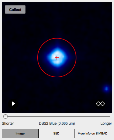 So what’s SIMBAD good for? Well, if your DiskDetective object is relatively bright, e.g. it looks like the image is saturated like the depicted here, or surrounded by its own diffraction spikes, then it will probably give you a reliable classification in one shot. You can quickly find out if your object is a star–and crucially, find out if it’s a star with a known disk! Just look at the “References” on the SIMBAD page, and you can browse the literature on the object, and check for papers about Debris Disks or Herbig Ae stars or T Tauri stars for example. If you do find an object with a known disk, mention it on Talk! Because then we all get to do a little jump for joy, because it shows DiskDetective is working as it should.
Then, once you have discovered a fainter good candidate on DiskDetective and checked the location of the SIMBAD object (e.g. from the “dist(asec)” column), and you’re sure it’s in your red circle, you can use SIMBAD to tell you lots of interesting information about it. For example, the “Gal coord.” on SIMBAD are the Galactic Coordinates. They tell you where your object is on the sky compared to the Galactic plane; the second coordinate tells you how far from the plane it is (from 0 to 90 degrees). Disks are often clustered into groups–and one goal of DiskDetective is to find more of these groups based on the coordinates and the proper motions, also listed in SIMBAD. (We’ll talk more about that later!)
SIMBAD also sometimes lists measurements of how bright an object is at wavelengths we don’t normally include in DiskDetective. These can help us improve the SEDs we have–once we have found a good candidate. (We’ll get into that later too.)
We included the SIMBAD links because while you’re doing your detective work, SIMBAD can give you some useful clues. It may even help you come up with your own research ideas. Just remember that ultimately, your goal as an astronomer is to improve and augment the data in SIMBAD, not to trust it blindly.
“I never guess. It is a shocking habit,—destructive to the logical faculty.”
Marc Kuchner
@marckuchner
Disk Detective and Planet Hunters
A few folks have asked us: what’s the relationship between Disk Detective and Planet Hunters? Planet Hunters, of course, is the Zooniverse citizen science website that invites users to examine data from NASA’s Kepler mission to search for extrasolar planets.
The success of Planet Hunters helped inspire us to launch Disk Detective! But beyond that, there are several scientific connections between the two projects. Both are about extrasola r planets. As you probably know, in Planet Hunters, users look at measurements of a star’s brightness, checking for sudden dips that could indicate a planet crossing in front of the star (called “transits”). In Disk Detective, we search for the homes of planets: stars surrounded by disks where planets form and often dwell.
Let’s talk more specifically–about what stars the two projects have in common. First of all, the data from the WISE mission that we’re examining at Disk Detective covers the whole sky. So it overlaps with everything, including the part of the sky that Kepler/Planet Hunters has already studied and whatever parts of the sky Kepler will image in the future. Indeed, the part of the sky Kepler has already examined has already been searched for disks at least once; Samantha Lawler and Brett Gladman claimed to find eight debris disks around stars with Kepler planets in 2012, using data from the WISE mission. However, further studies of the Kepler field were unable to replicate this result. The map above illustrates the current Kepler field, mostly located within the constellation of Cygnus.
But there will be more such Kepler/WISE disks for us to find via Disk Detective and Planet Hunters. For one, both the Kepler and WISE databases have improved substantially since that work was done. Kepler has found more transiting planets, and WISE scanned the sky again, leading to the new ALLWISE data release this fall.
Moreover, plans are afoot to extend the Kepler mission. The extended mission, called “K2” will search for planets in a different region of sky, near the plane of the Earth’s orbit. Here at Disk Detectives, we will already be searching that region for disks. And I’m pretty sure the new K2 data will be searchable at Planet Hunters as well.
So stay tuned–and keep digging for new disks! You might find one around a star that Kepler has already found planets around, or that it will find planets around soon. And even if there is not a direct match, we still learn by combining the statistical information from both surveys about how and where planets form.
“It has long been an axiom of mine that the little things are infinitely the most important”
Marc Kuchner
Seven Hundred Million Sources. Four Hundred Disks.
It was the curly-haired Dr. David Leisawitz who first told me about the WISE mission. I remember sitting in his office in front of a giant black-green-magenta sky map while he described how the WISE mission would find amazing kinds of disks: disks hosting young planetary systems, disks in old planetary systems, all kinds of exotic phenomena.
He told me how the science team was combing through the data right now by computer to find these disks. But every source had to be verified by eye.

I started wondering: is it possible that folks are going about this backwards? What if we could check through the whole WISE catalog by eye, right off the bat? What would we find then?
I made some quick estimates of how many disks could be find in the database that others had not already found by computer. The WISE mission observed more than 747 million sources all around the sky. My calculations told me that if we went through the catalog using the amazing power of human vision right off the bat, we could find almost 400 debris disks among this sample that nobody else could find. That’s not to mention all the other kinds of disks whose numbers I couldn’t calculate: protoplanetary disks, transitional disks, disks around white dwarfs and other evolved stars. And there could be other kinds of fascinating objects to find lurking in the data: Kardashev Type III civilizations, metal poor stars, planetary nebulae—
But I still wasn’t confident in the idea. So I called up Drs. Debbie Padgett and Luisa Rebull, who were also leading large efforts to find disks with WISE. Debbie discovered a spectacular example of a debris disk that in Hubble images resembled a giant skinny V, probably sculpted by a hidden planet. Luisa had been scouring star-forming regions, finding protoplanetary disks. And once again, in both Luisa’s and Debbie’s WISE searches, every source had to be verified by eye.
The next step was obvious; we wrote the Zooniverse folks and began working on a site. Fast forward through a few years of planning. Now David, John, Debbie and Luisa and I have joined with Dr. Mike McElwain and other experts to become the Disk Detective science team. A few more months of site development and here we are on launch day, ready to work with you, ready to find some disks that nobody else will spot–thanks to your eyes.
So let me take this chance to say that we can’t wait to meet you. I hope you are patient and determined, because it won’t be easy. But I think the chance to discover a new disk—a whole nascent planetary system—in one shot like this is worth the effort. And who knows what else we will find lurking in the spectacular WISE database, the deepest all-sky infrared survey every undertaken?
Thank you for joining us at Disk Detective. Good luck, and remember that the world is full of obvious things that no one ever observes.
Marc Kuchner
@marckuchner
