
Our New Paper is Out!
Good news, everyone: our latest paper from Disk Detective has just been accepted for publication in the Astrophysical Journal! You can read it on the arXiv now. In it, we estimate the number of disks we expect to find in Disk Detective, and present over two hundred new disk candidates that have received high-resolution follow-up imaging.
Disk Detective is designed to identify new disk candidates in the AllWISE catalog by eliminating false positives. Because we have such a large catalog and so many classifications that have been made so far (keep them coming!), we can get some statistics on how many objects are false positives, and use that to estimate the number of disks we expect to find. We can also break this down by what kind of false positive we find, and where in the galaxy we find it.

Objects as a function of Galactic latitude. Most objects are in the Galactic plane, and most of those objects are multiples.
In general, “multiples,” objects for which a majority of classifiers clicked “Multiple objects in the Red Circle,” are the most common type of object–more than 70% of the objects in the catalog! Only about 8% of objects are classified as “None of the Above/Good candidate” by a majority of classifiers. These occur most often in the Galactic plane, as you’d expect–if there’s more stars in the Galactic plane, you’d expect to get more disk candidates there. However, multiples become much more common in the Galactic plane, as well–the multiple fraction in the Galactic plane is over 70%!
We looked to see the multiple fraction (the fraction of objects in a given range that were multiples) as a function of Galactic latitude. We expected that these would be most common in the Galactic plane, and fall off as you got further away from it. We found instead that while for the most part this is the case, there’s an additional peak between -30 and -35 degrees Galactic latitude.


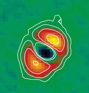
So we looked at the multiple fraction as a function of both Galactic latitude and longitude, as shown on this heatmap (brighter = higher multiple fraction), and found that most of those multiples outside the Galactic plane occurred at the same Galactic latitude as the Large Magellanic Cloud–we have multiples caused by stars in nearby dwarf galaxies, too.
In addition to the website classifications, we also review our objects in the literature to ensure that we’re not identifying things that are known to be non-disk sources (like background galaxies). This eliminates an additional 14% of our objects, the remainder of which becomes DDOIs.

Objects with high-resolution follow-up as a function of Galactic latitude. Unlike with the website classification data, there’s no significant difference between in and out of the Galactic plane.
We took high-resolution images of 261 of our DDOIs to see if we could identify faint background objects, fainter than would be detectable in our survey data but bright enough to produce a false positive at W4, using the Robo-AO instrument while it was at Palomar, and RetroCam on the Irenee R. Dupont telescope at Las Campanas Observatory in Chile. (I wrote about my observing experience at LCO here.) We included some volunteers from our advanced user team in the analysis of this data–they’ll have a blog post up on the details of what they did soon. Overall, we found that 244 of the 261 objects were good disk candidates once faint background objects were taken into account.
Combining all of these, we estimate that only 7.9% of all infrared excess candidates in AllWISE are or will be good disk candidates. That means that we expect to find 21,600 disks in AllWISE, almost double our original estimate!

Estimated false positive fraction for several surveys. Surveys that visually inspect the data (blue) have lower expected false positive rates than surveys that don’t (orange).
We were able to use our false positive rates to estimate how many false positives appear in published disk searches. Many surveys do a good job, but have some false positives due to objects only detectable in high-resolution imaging. Some larger searches, however, seems to be riddled with false positives, including the McDonald et al. (2014) and (2017) searches, and the Marton et al. (2016) search. These searches don’t include a visual inspection of the images, and thus are likely to have high rates of false positives due to multiples at the minimum.
We were also able to leverage the knowledge base of our Disk Detectives to analyze the M dwarf disk candidates of Theissen & West (2014). M dwarf disks are key targets, because very few have been found, despite the abundance of M dwarfs nearby. The advanced user team got together and found a way to analyze the targets as if they were Disk Detective objects (more on this in their blog post coming soon). We found that only 13 of the candidates from Theissen & West (2014) had high enough signal-to-noise for the Disk Detective methodology to apply. Advanced users found flaws with all thirteen, making all of them false positives.

An HR diagram of our candidates with parallaxes from Gaia. Color of each point indicates the disk temperature, while size of each point indicates the strength of the infrared excess. This plot shows that while most of our objects lie on the main sequence (like our Sun does), many others lie off of it. We think that most of the ones off the main sequence are primordial disks.
Finally, we presented a list of 244 disk candidates with follow-up high-resolution imaging, 213 of which are new discoveries by Disk Detective. These seem to be split evenly among debris and YSO disks, though some of those YSO disks could potentially be “extreme” debris disks, which are thought to result from collisions of terrestrial planets. We made some further interesting discoveries among these:
- We found that twelve of our new disks were in comoving pairs (that is, another star nearby to them has similar motion), providing further support to the hypothesis that warm circumstellar dust is associated with binary systems.
- We made the first identification of 22-micron excess around two stars that are known to be in the Scorpius-Centaurus young association, and identified known disk host WISEA J164540.79-310226.6 as a likely member of Sco-Cen, based on its motion through the sky. By identifying these targets as members of Sco-Cen, we give them likely ages, letting us put these on timelines of disk evolution.
- We found thirty-one disk candidates within 125 pc, including 27 debris disks. These are good targets for both direct imaging exoplanet searches, and spatially resolving the disk itself in scattered light–making these targets optimal for observation with the James Webb Space Telescope.
And there’s still more work to be done! We recently hit 76% complete (that is, 76% of all our targets have enough classifications to be retired from the website), but that leaves more than 60,000 excesses to evaluate with your help. We now know how many objects we’re going to find–now it’s our job to finish finding them.
Examples of SEDs
As we discussed in an early blog post, the SED (Spectral Energy Distribution) is a plot of how bright an object is are as a function of wavelength. You can find each object’s SED on its Talk page.
Tadeáš Černohous (TED91) put together a wonderful collection of some of the different kinds of SEDs that you’re likely to encounter on Disk Detective. Nice work, TED91! Here it is for your delight. I added a few comments here and there. –Marc
Early Type Stars (Debris Disks)
These stars are as hot as the Sun or even hotter, and generally have spectral types B, A, F or G. (Type O is even earlier than that, but these very massive stars are rare.) The SEDs for these stars are nearly straight, downward-sloping, lines because of the Rayleigh-Jeans law. You’ll notice however that the very last point always falls slightly above the straight line; that’s because all the objects in Disk Detective were pre-selected for this property. This “infrared excess” is a sign that they might be surrounded by a disk, which glows only at these longer wavelengths.

AWI0006207, AWI00062ka, AWI00062aj, AWI0004y3p
Late Type Stars (Debris Disks)
These are stars of spectral type K or M, which are cooler and don’t emit as much at 1 micron as a the early type stars. You’ll see that the first point of the SED is a bit lower for these objects. The physics of this phenomenon is the Wein Displacement law; the peak of the blackbody curve shifts to longer wavelenegths for cooler objects.
Another effect that can cause the first few points of the SED to drop is interstellar “extinction” or more specifically, interstellar “reddening”. That’s when interstellar dust between the star and the Earth absorbs some of the light at the short wavelength end of the SED.

AWI0005cm2, AWI0005mue, AWI0005m8k, AWI0005ag0
More examples
Young Stellar Objects (YSOs)
YSOs generally have more infrared excess than debris disks, and the excess kicks in at shorter wavelengths, even as short as K band. Many YSOs are also reddened by interstellar dust. The SED’s of these objects sometimes may look similar to those of Active Galactic Nuclei (AGN) and dusty red giant stars; it’s hard to distinguish among them. If you aren’t sure which one it is, try to find some information on SIMBAD or VizieR.

AWI0005wau, AWI0002ddn, AWI0002p0g, AWI0005wal
Saturated stars
See that point at 3 microns (fourth point from the left)? It’s “lower” than it should be. That sometimes happens when the light from a bright object “saturates” the detectors in the WISE 1 band. Most often, when you see this in the SED, you’ll also see that the WISE 1 image looks very misshapen or displaced from the crosshairs. These objects are NOT good candidates.

AWI0005ywh, AWI0005yuk, AWI0005x81, AWI0005zgc
Galaxies
The spectral distributions for galaxies can contain several components: stars of different types as well as dust at various temperatures. Moreover, galaxies can be redshifted by the expansion of the universe, a process that shifts the SED to the right, sometimes even halfway across the plot. We aren’t interested in these objects in this phase 1 of Disk Detective, though we might be in the future.

AWI00009x3, AWI0000fsq, AWI00062j8, AWI0000an0
Quasars and Active Galactic Nuclei (QSO and AGN)
These objects may look like stars to you at first glance, because they often appear as a point sources of light. But these SEDs are clearly very different from those of stars. This is one of the ways SEDs can be useful! Quasars and AGN are also classes of objects we aim to discard in phase 1 of Disk Detective.

AWI00000t3, AWI00005z0, AWI00001hs, AWI00001m3
Planetary nebulae
Planetary nebulae have nothing to do with planets. They are clouds of gas and dust belched out by an old red giant star. These objects are fascinating–but for the purposes of Disk Detective they are trash.

AWI0002dbc, AWI0005duo, AWI00006ju, AWI00059t3
Please note that all of these are just some common examples. The SEDs may be different from case to case, especially when those objects are somehow contaminated or blended.
A Dwarfs and K Giants
A list of 102 interesting objects that you helped pick for follow up (let us call them Disk Detective Objects of Interest, or DDOIs) shows that many of the stars with disks we locate will be A dwarfs or K giant stars. We don’t yet know all the spectral types of the DDOI stars precisely, but you can see the distribution of the types we do know in the figure below. The peaks correspond to A dwarfs and K giants.

Distribution of DDOIs according to spectral type. The two peaks at AV and K show that most stars hosting disks in our list are stars of type A and K that are about twice as massive as our Sun.
So what are A dwarfs and K giants? “A” dwarfs are very hot, fast spinning and blue stars that are younger and brighter than “G” stars such as our Sun. The bright stars Sirius and Vega are some well known A dwarfs. Many of the best studied debris disks are around A dwarfs.
What are these “K giants”? K giants and A dwarfs are two sides of the same coin. Let’s talk a bit about the life cycle of a typical star.
Most ordinary stars like our Sun burn hydrogen fuel for many millions of years. Once all the hydrogen is used up however, the star balloons in size and becomes a red giant. In the far future when our own Sun becomes a red giant, it will become so big that it will swallow up Mercury, Venus and possibly the Earth. Giants also tend to steadily lose a lot of their own mass all the time. This is because hot winds are blowing off the gas that is part of the star. (This hot gas is tricky because it might be mistaken for a dusty disk)
K giants are former A stars that have evolved for hundreds of millions of years. Like the sun, they have burned through their hydrogen, and ballooned up in size. Both A and K stars are about twice as massive as our Sun.

Left: Artist’s impression of Sirius, and A dwarf. Credit: NASA, ESA, G. Bacon
K giants are also really interesting because Jupiter-sized exoplanets orbiting these old, giant stars have been found to be more common than Jupiter-sized exoplanets orbiting less massive stars that are still on the main sequence. These exoplanets around K giants have been found by the popular radial velocity (Doppler shift) method.
Also, some of these K giants have debris disks, sometimes even dustier than their younger counterparts. This is surprising, because giants are very bright and light from the star exerts radiation pressure on small dust particles that ought to blow the dust away, or cause them to slow down and spiral into the star and be swallowed up.
So where is the dust around these K giants coming from? Nobody really knows yet, but there are several hypotheses. One is that dust is coming from the star itself. Another is that the dust is in fact interstellar dust in our galaxy. A third is that giants are breaking up more comets. Whatever the cause, we have a lot of K giants in our list of DDOIs that potentially have dusty disks–so once we can follow these up with telescopes we will be able to help solve this mystery.
Dawoon Jung (@dirkpitt2050) is a graduate student at the International Space University currently at NASA Goddard Space Flight Center doing a summer internship with the Disk Detective team. He was born in Korea, and is interested in exoplanets and space flight.
Herschel image of κ Coronae Borealis 31.1 parsecs away. This K giant is about twice as massive as our Sun. The red regions correspond to dust orbiting the star. Interestingly, this star also hosts at least one exoplanet with a mass of about 2 Jupiters. Credit: Bonsor et al. 2013.
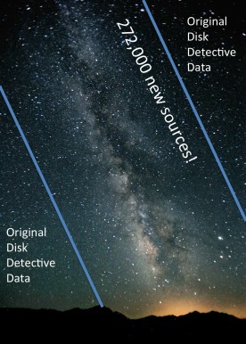
Good News Everyone! 272,000 More Subjects
January 28 we launched DiskDetective with a first batch of about 32,000 sources to classify. Of these, 20,000 have been in rotation at any given time. That’s a lot of astronomical data–and a lot of flipbooks to look at.

Well, it completely shocked us when we heard in March that some folks were seeing repeats–meaning that they had already classified more than 20,000 subjects! Now, we had always planned to have many more subjects than that in Disk Detective. But at that point, we were still in the process of downloading the data from the NASA/IPAC Infrared Science Archive onto a hard drive on Marc’s living room carpet, a process that took about a month. So we weren’t ready to put any more data online to keep all our detectives detecting.
The figure below shows the distribution of the J magnitudes of the sources with excess emission at 22 microns that WISE made really high quality images of (specifically ones from Southern Galactic latitudes, but that doesn’t matter). The total distribution, shown by the black curve, has two peaks, one around J=9, the other around J=16.
What is the meaning of these two peaks? Could it be two different kinds of sources?
The red and orange curves tell the rest of the story. The red curve shows the numbers for just those sources close to the Galactic plane. The orange curve shows the numbers for the remainder of the sources–those far from the galactic plane. Dividing the sources up in this manner shows that the second peak is mostly due to distant galaxies.
At low galactic latitude, dust from our Galaxy, the Milky Way, obscures most galaxies external to our own. So we know that the objects shown by the red curve–most of the peak at J=9–are stars (and maybe stars with disks). At high galactic latitude, the opposite is true. The objects shown by the orange curve should be mostly galaxies. That’s the peak at J=16.
For now, we’d like to skip the objects that are mostly galaxies (orange curve) and concentrate on the objects that are mostly stars (red curve). The orange and red curves cross at about J=14.5, so we decided to put aside the objects with J > 14.5 for now. That means this new batch of data should have fewer galaxies in it than the old batch–and more of those delicious disks!

What are we doing with the sources with J magnitude >14.5? Don’t worry, we’ll be putting them to good use. Our colleagues have suggested that hidden among those fainter sources could be Kardashev Type II and Type III civilizations. So once we’re done with this new batch of sources (roughly in 2017), we’ll start looking at the fainter objects–looking for signs of extraterrestrial intelligence. In fact–you may have already spotted some in the first batch of data. (They look just like debris disks and very red galaxies). Stay tuned!
Follow-Up Observing Begins!
In our last blog post, we invited you to submit interesting targets to follow up with the Tillinghast 1.5m telescope at Mt. Hopkins this spring. Thank you to jessicamh, Gez Quiruga, arvintan, kmasterdo, silviug, wtaskew, cpitney, Pini2013, Ted91, Vinokurov, michiharu and everyone else who submitted targets! Thanks to your help, we picked out 102 objects to follow up this spring. The observing starts tomorrow night.
And guess what? We’ve got more follow-up observing planned for the fall semester, and also for the Southern hemisphere, with help from our new collaborators, Luciano Garcia and Mercedes Gomez from Observatorio Astronómico de Córdoba and Christoph Baranec from the University of Hawaii.
So we’re keeping that target submission form open. From now on, whenever you find an interesting target, anywhere in the sky, feel free to submit it.
And now that we’ve been through this process, I can better explain how we decided what to follow up this time. This part of the blog post is going to be a bit technical–so feel free to skip it, or ask us for more info if you get tripped up by the jargon.
We started by searching SIMBAD and VizieR for information on each object, keeping the search radius to 0.2 arcminutes. These are the kinds of objects we most want to follow up:
Main sequence stars (aka dwarfs)
Luminosity Class IV stars: A IV, F IV, G IV, K IV, M IV.
A III, F III, G III and K III stars
T Tauri stars and Herbig Ae stars
white dwarfs
objects with distance < 200 parsecs
objects with proper motion > 30 milliarcsec/year
shell stars
We generally don’t want to follow up:
M giants
Cepheids
Be stars
galaxies, Active Galactic Nuclei
blends (i.e. two objects so close together that we can’t analyze them separately)
eclipsing binaries
O stars
supergiants
Also mixed in the lists of possible targets were:
binary stars
known disks
and plenty of objects where we can’t tell what it is
These objects went onto a “Maybe” list, to be followed-up as second priorities.
We could read some of this information from the SIMBAD spectral type. The quality of this information varies, and the SIMBAD spectral type includes a data quality letter (A,B,C,D, or E) where A is the best. Since the purpose of this observing run is to weed out blends and to get more accurate spectral types, we figured it was OK to look at objects where the spectral type quality was poor. But we threw out objects classified in SIMBAD or VizieR as M giants, Cepheids, Be stars, galaxies, Active Galactic Nuclei, eclipsing binaries, O stars or supergiants.
The most common contaminants are M giants and supergiants. We want to avoid those. But some M stars are main sequence stars (dwarfs). Like this one: AWI00003dm Disks around these M dwarfs are rare and interesting and worth extra points! So we must be careful weeding out the M giants and supergiants.
M giants are sneaky! They come with many different labels in SIMBAD and VizieR: Long Period Variables (LPVs), SR+L, Slow Irregular Variables, Miras, Semi-regular Variables, Semiregular pulsating Variables, Carbon stars. All those are kinds of M giants/supergiants and they tend to make their own dust, so we can’t use dust around them as an indicator of a planetary system. We’re not following them up.

M dwarf disks are exciting but rare. Here’s a Hubble picture of one around a star called AU Microscopii.
Sometimes you can spot an M giant even when there’s no known spectral type. For example, subtract the V magnitude from the K magnitude. If V – K > 3.29, you’re looking at an M star. Then, if a star has a measured distance of thousands of parsecs, you can bet it’s a giant or supergiant. So we declared some objects to be M giants based on color and distance. A real M dwarf is so faint we can only see it if is much closer than 100 parsecs.
Here’s more information about how to guess a star’s spectral type based on its color: http://www.stsci.edu/~inr/intrins.html
If you know you’re looking at an M star, another good clue that it’s a giant/supergiant is if it is highly variable (e.g. amplitude more than one magnitude). So we looked up the variability amplitude for our targets in VizieR as well.
For an M star with no parallax measurement and no variability measurement, it can be hard to tell if you’re looking at a dwarf of giant or supergiant. So I put objects like that on the “maybe” list.
And finally–all the subjects on Disk Detective are preselected to have a certain degree of redness (we require the WISE 4 magnitude to be at most the WISE 1 magnitude – 0.25). But that’s not sufficient to find M star debris disks, since M stars are so cold, and therefore intrinsically red colored. We had to additionally weed out M stars with WISE 4 magnitude > WISE 1 magnitude + 1.0. (I know that sounds terribly confusing–it’s confusing because in the astronomical magnitude system, brighter objects have lower magnitudes. But adding this second criterion says that we are being more demanding when it comes to M stars in terms of how much brighter they need to be in the WISE 4 band than the WISE 1 band.)
Whew—that’s a lot of detail, I know. But now you can see why we try to weed out all those blends and multiples etc. using the handy animated flipbooks on the DiskDetective site before we start all the detailed research on each one.
Here are all the objects on our current version of the follow-up list for the Tillinghast 1.5 m for this spring, below (this list includes the maybes). Thanks again for all your hard work. And keep our fingers crossed for good weather at Mt. Hopkins!
Marc
| Zooniverse ID |
| AWI0000bs0 |
| AWI0000tjx |
| AWI0000gjb |
| AWI0000fye |
| AWI0000kg4 |
| AWI0000ojv |
| AWI0000tz1 |
| AWI0000u8s |
| AWI0000uj2 |
| AWI0000uji |
| AWI0000w9x |
| AWI0000ibq |
| AWI0000v1z |
| AWI00006nk |
| AWI00000wz |
| AWI0000tgc |
| AWI00002ms |
| AWI0000cot |
| AWI0000nwt |
| AWI00002zo |
| AWI0000m2p |
| AWI0000ns8 |
| AWI00004o8 |
| AWI000050r |
| AWI0000hjr |
| AWI000048c |
| AWI00005uf |
| AWI00000o6 |
| AWI00001l8 |
| AWI00002yt |
| AWI0000hog |
| AWI0000kk6 |
| AWI0000eg6 |
| AWI000004g |
| AWI00007qu |
| AWI000001j |
| AWI00001q1 |
| AWI00005xz |
| AWI00006bt |
| AWI00004qc |
| AWI00000zp |
| AWI0000kgo |
| AWI00007dp |
| AWI00000om |
| AWI00006dp |
| AWI0000149 |
| AWI000011b |
| AWI0000l8w |
| AWI0000us7 |
| AWI0000gz9 |
| AWI000028h |
| AWI0000vk9 |
| AWI0000jo8 |
| AWI000015r |
| AWI00000au |
| AWI000066t |
| AWI00002xh |
| AWI00006kc |
| AWI0000632 |
| AWI0000np1 |
| AWI00002fw |
| AWI00006p0 |
| AWI0000ajw |
| AWI00007i1 |
| AWI000047d |
| AWI0000tpu |
| AWI0000qxd |
| AWI0000hat |
| AWI000055c |
| AWI0000wip |
| AWI00006b3 |
| AWI0000tsh |
| AWI00002hx |
| AWI000054k |
| AWI00001sw |
| AWI0000r07 |
| AWI0000t35 |
| AWI0000a7e |
| AWI000019z |
| AWI0000s7e |
| AWI0000wqx |
| AWI00005x2 |
| AWI000042e |
| AWI0000aoe |
| AWI00004ox |
| AWI00000lj |
| AWI00000my |
| AWI000034n |
| AWI00004c1 |
| AWI00005ko |
| AWI00006hl |
| AWI00006nb |
| AWI00007fu |
| AWI00007ne |
| AWI0000c02 |
| AWI0000l70 |
| AWI0000s8t |
| AWI00006m2 |
| AWI000072k |
| AWI0000qnj |
| AWI000016c |
Chasing Dust Around Dead Stars
The typical place to find dusty debris disks is orbiting around ordinary stars like the Sun, or younger stars that are in the process of forming terrestrial planets. But some dusty disks that you might spot in Disk Detective surround tiny, exotic dead stars called white dwarfs.

An artist’s impression of the evolution of a planetary system from middle-age to the star’s eventual death as a white dwarf. In the process, surviving asteroids can form a dusty disk around the white dwarf. Credit: Mike Garlick
Most ordinary stars like the Sun will end their lives by bloating up into red giants. The cores of the red giant stars are balls of mostly carbon and oxygen, the spent fuel of the nuclear burning that powers the star. Red giant stars blow away much of their mass in winds, and eventually become stripped down to naked cores. It is called a white dwarf when those winds are done blowing, and there is nothing left of the star but its carbon and oxygen core covered with a very thin layer of hydrogen gas. White dwarfs are just a bit larger than the Earth in diameter, though they generally weigh around three-quarters as much as the Sun!
For a long time people thought that the process of stellar evolution into white dwarfs meant certain death for any planetary systems that might orbit the original stars. Indeed, inner terrestrial planets may indeed be destroyed by this process. But large asteroids, giant planets, and potentially even icy bodies might survive if they are big enough and far enough away to weather the drastic changes that a star goes through. Astronomers are now studying the nearest white dwarfs for signatures of these possible surviving planets.
One telltale signature is the presence of dust orbiting a white dwarf. If we look at a white dwarf in infrared light, with a telescope like the WISE telescope, a dusty white dwarf will be brighter there than at shorter wavelengths, just like the targets of Disk Detective. Thanks to many observations of white dwarfs with the Spitzer Space Telescope, WISE, and NASA’s ground-based Infrared Telescope Facility, we have discovered a few dozen dusty white dwarfs in the last 10 years. We believe the dust around these stellar ghosts comes from asteroids kicked too close to the central white dwarf by a larger planet. When this happens, the asteroid shreds apart much like Comet Shoemaker-Levy 9 did when it collided with Jupiter in 1994, and the pieces of it form a disk around the white dwarf. The size of the disk is not much larger than Saturn’s rings.
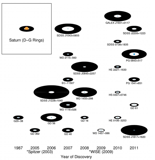
A collection of nearby white dwarfs and their accompanying dust disks. The dust disks are drawn to scale with Saturn’s rings. Credit: John Debes
Dust from the disk continues to rain down on the white dwarf surface in the form of atomic gas. Astronomers can measure the composition of this atomic gas—and thereby that of the dust—by taking optical and ultraviolet spectra of the white dwarfs. Just like characters from TV shows like CSI break materials found in a crime scene down to their component elements to identify them, astronomers compare the pattern of elements to Solar System bodies to understand the origin of the dust. Sure enough, they look just like asteroids in our own Solar System.
By chasing this elusive dust around dead stars, astronomers are using these clues to piece together the chemical history of terrestrial planet formation around other stars using the shredded remnants of exo-asteroids. The information they gain from studying white dwarfs might be able to tell us whether terrestrial planets have similar properties to our own Earth.
John Debes
That’s no moon…
A very common question here in Disk Detective is, hey, is that a planet? A disk? A moon? Those are exciting things to think about. Let me skip to the punch line: no, sadly, we can’t see planets, disks, or moons in the Disk Detective images. But let’s talk more about distances and angles, and I’ll try to better explain what we can and can’t see.
From this earlier post, we know that the overlays on the images in Disk Detective, in units of arcseconds, are :
- Red Crosshairs: 2.1 arcseconds across
- Red Circle: 10.5 arcseconds radius
- Disk Detective image: 60 arcseconds across
(If you need a refresher on what an arcsecond is, try this post from another site.) The overlays aren’t the only thing with angular scales that are important here. The original pixels in the DSS are about 1.7 arcseconds; the pixels in 2MASS are about 1 arcsecond, and the pixels in WISE are about 1.4 arcseconds.
OK, so physically, what do all of these angles mean? We could start with something at least somewhat familiar — the Moon is about half a degree in diameter, or about 30 arcminutes. Here is a post from another site that has lots more good information tying angles on the sky to familiar objects (like your finger).
Now, let’s start applying these ideas. The stars that are in Disk Detective appear to be relatively large on the screen. But are they really that large on the sky? Proxima Centauri, the closest star to the Sun, is about 4.2 light years away. In 2002, the VLT measured the diameter of this star to be “1.02 ± 0.08 milliarcsec, or about the size of an astronaut on the surface of the Moon as seen from the Earth (or a head of a pin on the surface of the Earth, as seen from the International Space Station).” (quote is from the press release in the link.) Let me emphasize this: MILLIarcseconds, so about 0.001 arcsecond. The Disk Detective crosshairs are 2.1 arcsec, and the pixels in those images are between 1 and about 2 arcseconds. Proxima Cen is the closest star to us, and it is a fraction of a fraction of a pixel in the Disk Detective images. We can’t typically determine sizes of other stars with most of our current instrumentation. The only people who can get the sizes of other stars right now are people who use optical or infrared interferometers, and only for targets that are relatively close and relatively bright. So the stars in Disk Detective only appear to be measurably large on the image, because of the way that the telescope+detector responds to the source of light.
Let’s go further, and put an imaginary disk around Proxima Cen that is the size of our Kuiper Belt. Making some simple assumptions, I get that it would be about 30 arcseconds across, so half the size of the Disk Detective image. But it would be impossibly faint at all of these bands, very difficult to see in these relatively shallow images (by which I mean ‘short exposure time’ such that we only see the brighter things). And we are still working with just the very closest star.
A relatively nearby star with a real (not imaginary) disk is Beta Pictoris, at about 65 light years away. This star is also impossibly small compared to the pixels here. Its disk, though, is ENORMOUS, 5 times larger than our Solar System. I get that it is about 102 arcseconds across, larger(!) than our Disk Detective images. BUT, it too would be impossibly faint, very difficult to see in these relatively shallow images, and in fact unless you found a way to block the light from the central star, it would be impossible to find the disk. This is what astronomers really do – we have a special shade that blocks out the light from the central star so that we can stare for a long time and collect light just from the disk. Planets (or Moons for that matter) are far, far fainter than the disk, and we still need to block the light from the central star (and make some good wavelength choices to maximize the brightness of the planet compared to the star/disk). Even when we do that, though, one of the planets found in Beta Pic’s disk is 0.4 arcseconds away from Beta Pic. …Aaaaand, now, we’re back to fractions of pixels in Disk Detective, even if we could block the light from the central star.
And it gets worse! There is this blog post on issues of spatial resolution in Disk Detective. The WISE spatial resolution is ~6 arcseconds. SIX ARCSECONDS. When you get to 22 microns, it’s TWELVE ARCSECONDS. That means that if two things are 12 arcseconds or less, WISE at 22 microns can’t tell that there are 2 objects. (That’s why we ask you in Disk Detective to indicate if you are seeing 2 objects in the shorter wavelength images.) The rest of WISE can’t tell if there are two objects that are 6 arcseconds or less apart. The spatial resolution of the DSS and 2MASS is closer to 2 arcseconds. So pixel size is rapidly overtaken by spatial resolution issues at the longest wavelengths, where the disk is brightest.
 At 25 light years, Fomalhaut is another relatively nearby star that has a disk. The Herschel observatory snapped a picture of it, but its eyesight (at longer wavelengths) is about 3-4x better than WISE at 22 microns. The dust’s light is also dependent on its temperature–cold dust will glow more brightly at longer wavelengths. Dust that is bright at 22 microns is typically much closer to a star. Even in the most optimistic case where you have a bright extended disk like Fomalhaut, it would barely peek out from behind the edges of the WISE “blob” (the response of WISE to the light from the unimaginably small point of light that is the star), shown in the upper left hand corner of the figure–the pictures of Fomalhaut as it looks at 25 light years and 160 light years are shown on the lower right of the figure, to scale on the sky with the WISE 22 micron PSF. See? Waaaay too small to be seen with WISE. And, at 160 light years, too small for Herschel too.
 What might WISE see with Fomalhaut? Using a rough model of the Fomalhaut disk and smearing it out with the WISE PSF, it might look like this, provided the entire disk was just as bright as the central star at 22 microns. BUT that is not really the case for Fomalhaut–the disk is at least ~40x fainter than the star at that wavelength. And it gets worse – most of the emission from Fomalhaut at about 24 microns does indeed come from a cloud close to the star; that part is 10x brighter than the total outer disk flux, but that’s still much fainter than the star.
But, wait, you say, you know you have seen pretty pictures of disks before in the media! Well, sometimes those are artist’s conceptions, where we are inferring the presence of disks from the excess of emission in the IR (“more IR than we think there should be”). Sometimes they are models of what people think these things must look like. None of the gorgeous images are from DSS, 2MASS, or WISE. And, yes, there are four famous disks that are nearby: Vega, Fomalhaut, β Pic, and ɛ Eri. Nearly all of the great images are of these four. There are another 8 debris disks that are further away than these closest four, but close enough that we stand a chance of getting images of them, so you may also have seen images of one of these 8. But there are only a total of 40 or so debris disks that are close enough that our current instrumentation can distinguish a disk from the central star, and sometimes it’s just barely distinguished, even when using the best tools available. And, especially then, it sure doesn’t look like a ring.
Distances to these objects matter, a LOT. The overwhelming majority of stars in Disk Detective are much, much further away than these 4, 12, or even 40 closest debris disks. The closest ones in Disk Detective are most likely at the very best 300 LY away. Even if we put a Kuiper Belt around such a star, it would be less than half a pixel across. Even if we put an ENORMOUS disk, like Beta Pic’s, around such a star, it would be about 2 arcseconds across, comparable to the size of a pixel in Disk Detective (and still impossibly faint compared to the brightness of the star). Remember that planets or moons are far, far, far fainter than the disk, and usually closer in than the full extent of the disk. So there is just no way that we can see planets or moons in the Disk Detective data.
If you find something that appears in the images of a target you’re looking at, and it is beyond the radius of the red circle, how far would it be from any given target? The circle is at 10.5 arcsec, and most of the questions I’ve seen on this topic are finding objects outside of that circle radius, so let’s call it about 20 arcsec. In the best case of our target being a star (1st assumption) that is 300 LY away (2nd assumption), and that the second thing is also a star (3rd assumption) at the same distance (4th assumption), that second thing is 0.03 light years away from the target object, or 45 times the size of our Solar System. That’s not a reasonable size for a disk around a star, much less a planet. And this is the best possible case, for the closest star in Disk Detective — most of the stars are much further away.
Disks and rings are MUCH smaller in size than the smallest detail that WISE can see at long wavelengths. Every known circumstellar disk is unresolved with WISE, including Beta Pic and the other 11 of the closest stars with disks. And if we can’t see rings or planets around these stars, we certainly can’t see moons around the planets, which are generally smaller than the planets. For example, the Earth’s moon is just about the size of the state of Texas–much smaller than the Earth.
The other objects that appear in the Disk Detective images, even within the circle, are other stars or galaxies that just happen to appear in the images. The chances of them being associated with each other (even as a binary star system) are extremely, extremely low. And they are not planets or moons around these stars.
Lots of people want to image disks and planets, though, and lots of people, especially at NASA, are working towards that goal. We are looking for new disks all the time, and using existing instrumentation where we can to image disks. But to get lots more images of lots more disks, we need special instrumentation (much of which is still being designed, including at NASA), we need to be observing at the right wavelength (e.g., pick one at which the disk or planet is likely to be as bright as possible), and have the star+disk be close enough to us that we can resolve it. The limits for “close enough” are moving out further and further every year as we develop more and better instruments to look for these things.
— @lrebull with help from @johndebes, @marckuchner, & D. Padgett
Spectral Energy Distributions (SEDs)
@ geckzilla asked on Talk:
I’m unfamiliar with SED diagrams. Could someone give me a few pointers? I read the short paragraph on the science page so I get the gist but I was wondering what some specific examples as they pertain to this project might look like.
SEDs are an important tool for recognizing and understanding disks. So I thought I might copy over here the answer I put there, and expand on it a little.
SED is an acronym meaning “spectral energy distribution”. So, it tells you where the energy is coming out as a function of wavelength (that’s the spectral part) from the combined light of whatever you’re looking at. By plotting up the energy emitted by an astronomical object, we can compare at a glance the emissions across a broad range of wavelengths. Does most of the energy come out in the UV, optical, or in the IR? The answer to that question can tell us something about what the object is.
For Disk Detective, we hope what we are looking at is {star+disk+anything else nearby including background sources} but it may very well be the combined light of a galaxy. The bands shown in Disk Detective come from optical (SDSS, DSS), near-IR (2MASS), and mid-IR (WISE). You can make an SED out of whatever photometric or spectral data you have on any given object (as long as the data are calibrated).
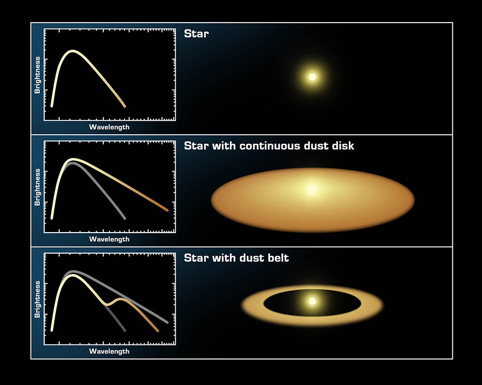
Stars without disks will look something like what physicists call a blackbody. That’s the top panel in the figure above. There is a mathematical description of this shape, but basically it describes the energy coming out from anything that is glowing due to heat – you, your toaster heating elements, an incandescent bulb, etc. The amount of energy emitted by an object at all wavelengths varies with the temperature of the object. Hotter objects emit more light at shorter wavelengths than cooler objects.
On the other hand, stars with disks have a little “extra” energy coming out in the IR – that is light from the star that is absorbed by the dust around it, which heats up and re-emits in the IR. That’s the bottom two panels in the figure above. At Disk Detective, we have pre-selected all the objects you will look at so their SEDs show a little “extra” energy coming out in the IR.
Once you look at a bunch of SEDs, you develop a calibrated eye for what works as a star+disk and what doesn’t. So you might want to take a look at these examples to get a better feel for what SEDs can tell you.
Examples:
- The diagram above, with some more explanation: http://www.spitzer.caltech.edu/images/2632-sig05-026-The-Invisible-Disk
- Another diagram showing the effect of small dust grains on the SED: http://www.spitzer.caltech.edu/images/1179-ssc2004-08c-Spectra-Show-Protoplanetary-Disk-Structures
- SED from a white dwarf with a relatively large excess: http://www.spitzer.caltech.edu/images/2054-sig09-002-Emission-from-the-White-Dwarf-System-GD-16
- SED from a star with just a little excess: http://www.spitzer.caltech.edu/images/3282-ssc2010-07a-Spectral-Signatures-of-Planetary-Doom
Hope this helps at least a little.
Luisa Rebull (@lrebull)
