
My Day at NASA Goddard Space Flight Center
Disk Detective Milton Bosch stopped by NASA Goddard Space Flight Center this month to meet with some of the science team and see the James Webb Space Telescope being built. What ended up happening that day we never could have guessed! Here’s the story, in his words.
My Day at NASA Goddard Space Flight Center
by Milton Bosch Nov.20, 2015
Greenbelt, Maryland has always held a special place in my heart and mind. I met and courted my wife there and lived three wonderful years in a unique New Deal era city in suburban Maryland outside Washington, DC. It has a lake and even camping at Greenbelt Park, part of the National Park system. Best of all, NASA in its wisdom had chosen Greenbelt as the site
for its first Space Flight Center. NASA Goddard opened on May 01, 1959. We had it all.
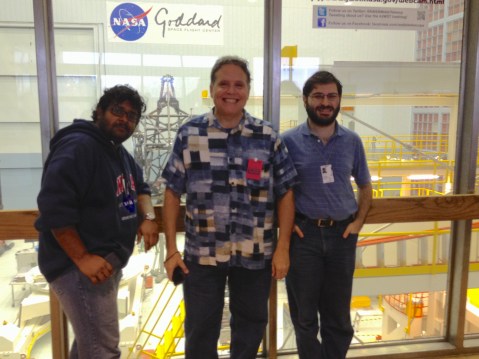
Shambo Bhattacharjee (left), Milton Bosch (center) and Steven Silverberg (right) at Goddard Space Flight Center, with the James Webb Space Telescope, under construction.
I’d always look at the guarded entrance across from our shopping center, and wonder, What is going on inside those gates? Really cool stuff, no doubt. That was in 1981; I was in medical school and there was almost zero chance I’d ever be invited there. Even after moving to California for residency training and my career in internal medicine, my NASA Goddard
memories were kept alive whenever I had a faint recollection. When a good friend named Willy got a job at Goddard as a machinist in 2010, the connection deepened a wee bit. I could picture myself inside if Willy could get permission to bring a visitor. That snippet of hope left when Willy left NASA Goddard after a couple years.
Fast forward: It’s now November 04, 2015 and I’m on a Google hangout call with the science team of Disk Detective, a citizen science project run by NASA. Months earlier, a NASA email arrived announcing a new citizen science project on January 30, 2014 , with a grant from The Zooniverse. Disk Detective’s goal was to locate protoplanetary disks – very early solar
systems – around young stars, and debris disks around more mature ones. I thought, “Discover new solar systems and planets and help learn how they form? I’m in!” I thought “in” was just doing classifications of objects, using the Disk Detective flip-book to triage them into two basic categories: a good candidate, or flawed (and reasons why). After doing many classifications came the invitation to become a superuser from principal investigator Marc Kuchner. As such, I learned how to navigate the astronomy catalogs, and choose promising objects for the main spreadsheet and hone my classifying skills. Step by step, with lots of mentoring and greater responsibilities, I was eventually asked to join the science team and here I was, sitting at my computer on November 5th for our weekly Google hangout with the science team.
I mentioned to Marc that I had won two free concert tickets to Madison Square Gardens for Nov. 7th, and would be staying near Greenbelt in Crofton, MD. Then Marc asked if I’d like to drop by on Nov. 6th for a tour of NASA Goddard Space Flight Center. Two days later I fulfilled my dream. What came later was a big surprise for everyone.

Milton Bosch and Shambo Bhattacharjee in Marc Kuchner’s office at Goddard Space Flight Center.
We started out with meeting everyone on the Disk Detective team at NASA Goddard. It was great finally meeting Marc Kuchner, PI, and graduate students Steven Silverberg and Shambo Bhattacharjee. We did a quick tour of the ground level, and then visited the offices of each. Then, upstairs to see the world’s largest clean room, where the James Webb Space Telescope (JWST) is under construction. We exited the elevator to discover a VIP tour in progress, and it slowly dawned on me that I was looking at North Dakota senator Heidi Heitkamp. She was not just any US Senator; she was a senator I liked and had supported her campaign. I whispered to Marc that I knew a bit about Senator Heitkamp, so he asked me to ask her a question about citizen science. I said, OK, and waited for my opportunity.
Just when it seemed like the right moment would never appear, I saw a raised hand asking if we could talk about citizen science. Senator Heitkamp walked over and introduced herself to each one of us, asking our names, where we lived, what our jobs were, and what we did before coming to NASA Goddard. She was pleased to meet a supporter from Napa, California. She wanted to know my journey from organic chemist, to medical doctor, to having to go on full disability, to finding and joining Disk Detective. So I told her my story of today being the fulfillment of a 34 year-old dream, all made possible by joining Disk Detective almost two years earlier, and a 1:20,000 chance of winning 2 free concert tickets to Madison Square Gardens.
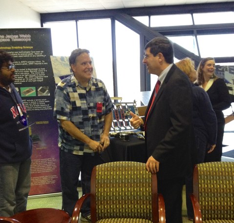
Milton meets Center Director Chris Scolese. Senator Heitkamp and Shambo Bhattacharjee are in the background.
While we talked, the cameras were snapping away and all-in-all, I think we got to spend 15 minutes on Disk Detective and citizen science. It was an unlooked-for opportunity to get the word out about Disk Detective and citizen science with one of our U.S. Senators and it could not have gone better. We were glowing for the rest of the day from the encounter.
Then the room cleared, and we got to see what we had come upstairs for: the James Webb Space Telescope under construction. (One of the goals of Disk Detective is to find targets to propose to observe with this telescope.) We could see the frame, the folded wings, and folded arm for the secondary mirror. On catwalks 80 feet above the crew sat a row of flat dewar flasks, each containing one hexagonal mirror. Launch date is less than 3 years away – October, 2018. Giant rolls of shrink wrap were placed all about for final sealing before JWST’s journey to the launch vehicle. I looked at everything in the room visible from our vantage point and then went downstairs and peeked through an entrance door window. No photos are allowed through that window, nor inside either.
Next stop was one of the “testing rooms”; though I’m sure it has a formal name. It had an 8 story high egg-shaped metal container, filled with liquid nitrogen for starters. Inside that was another cryogenic container filled with liquid helium. Every single piece, every instrument, every device must survive that environment before it can be trusted for launch. After all, they must function at extremely low temperatures. But more terrors awaited the equipment and instruments that go into space.
Nearby was a huge room with a centrifuge that dwarfed a blue whale. It was like the room where the centrifuge scene from The Right Stuff movie was filmed, but this centrifuge has a different purpose. In order to test equipment properly (not people), the centrifuge reaches up to 15 G’s of acceleration, helping insure against failure in the most stressful environments imaginable. Steven said it would tear a human to pieces.
Next door to that was a huge acoustic testing room with a 7 or 8 foot “tweeter” and a 12 foot “woofer” with a maximum combined sound intensity of 150 decibels. No humans are allowed inside that lethal chamber. An adjacent room held the machinery that powered the 150 decibel monster. A six inch hose for pressurized nitrogen powered the tweeter, and emitted so much of the simple asphyxiant that there is no admittance during testing. We paused our tour for a relaxing lunch in the cafeteria, and then filled time while Marc had teaching duties. Those duties now completed, we all met in Marc’s office, where all the Google hangouts take place (with other scientists joining from Adler Planetarium, The Space Telescope Science Institute, University of Oklahoma, and more).

Milton and Senator Heitkamp study a poster about the James Webb Space Telescope, while the cameras click.
We spent an hour discussing ways to improve our sound recordings and other technical issues, as well as more important problems, like finding a replacement llama doll for Marc’s very young son, should he lose his beloved cozy-coze. Then I was presented with a highly coveted Disk Detective coffee mug, and we took photos of a poster where my name appeared as co-author, alongside the names of five other citizen volunteers like myself. Then it was time to go.
It was a truly great day, full of the unexpected, and a real pleasure meeting some of the science team in person. Never give up on your dreams! Disk Detective will take you as far as you want go and has all types of support while you navigate the learning curve…all the way up to co-authorship of scientific papers.
Pictures from our Observing Run in Chile
Steven Silverberg from our science team just came back from South America where he went to observe some Disk Detective Objects of Interest with the DuPont telescope. Here’s his story.
We have a program to take high-resolution images in the near-infrared band (between the DSS “IR” band and 2MASS “K” band we use on the Disk Detective site) with the 2.5m DuPont telescope at Las Campañas Observatory, one of the premier observatories in the world. It’s similar to our follow-up program with Robo-AO; the images help us double check for background galaxies and stars that could be lurking very near to our disk candidates, so close to them that they wouldn’t appear in the data we already have. We have access to this telescope in Chile thanks to Johanna Teske, a member of our science team at the Carnegie Institution for Science. Because Johanna couldn’t go on the observing run this time, I went to South America. It was my first time outside the US–very exciting!
 The first thing that struck me were the spectacular views. LCO is 2,380 meters (7,810 feet) up in the edge of the Andes. For someone who grew up in the part of Texas that doesn’t have mountains, it was rather incredible.
My first night there was spent shadowing an observer for the Carnegie Supernova Project, an ongoing campaign to fully characterize the behavior of supernovae in multiple bands. Unfortunately, most of this night was wind-ed out. DuPont has a firm wind speed limit of 35 miles per hour; anything above that, and the dome must close.

Most of DuPont’s controls are handled by computer. However, one last panel from the original control board is used for operating the lamps used for calibrating the detector (the dials next to the LCD readout). The rest of the panel has been superceded by computer, hence all the “Do Not Use” signs.

One upside to going nocturnal for telescope time: you’re awake for amazing sunrises and sunsets. In this case, morning twilight on the mountains to the west.
 The most impressive feature of the observatory was the mountain on which the twin Magellan telescopes reside. These two telescopes, each 6.5 meters in diameter, loom over the observatory lodge. LCO will eventually (by 2025) be the site of the Giant Magellan Telescope, which (along with telescopes like JWST) could be used to image Disk Detective disks!
 There are two other major telescopes at LCO currently: the Swope telescope (in the foreground) and DuPont (centered), where we conducted our observations. These are the two oldest telescopes on-site; the Swope went on-line in 1971, while DuPont came on-line in 1977.
 Because of the timing of my visit (right around full moon), I was able to get some excellent images of moon-rise. This one was taken before my first night of observations, which (like the night prior) was mostly lost due to wind. However, we were able to get 19 objects imaged on night 1, despite losing several hours to wind.


The sunrises were absolutely beautiful while I was on-site. I enjoyed taking pictures of them. These are several different captures of the sunrise after night 1 of Disk Detective observations, taken from my room at the lodge.
 This was the view looking south from the lodge. The road below is the road back down the mountain from the site. GMT will be built on one of the mountains down here, to the left of this shot.
 This is how the observatory looked when viewing from DuPont. Magellan is in the background left; the Swope is in the middle.
 The road from DuPont back to the lodge. As one might expect for a mountain in the Atacama desert, the local foliage was rather sparse. The same weather conditions that lead to this sparseness make LCO an amazing site for astronomy.
 You could see some snow-capped peaks of the Andes in the distance, which were rather incredible to see in person (albeit not particularly close by).
 While on the mountain, I got to use a car reserved for DuPont observers. Having never driven on a mountain before, that was new and different…and a bit frightening. Especially driving down the road above at morning twilight, with limited visibility.
 The actual DuPont dome. It was quite big (as one would expect, to house a 2.5-meter telescope).
 The actual DuPont 2.5-meter telescope. Rather than use a (rather heavy and difficult to maintain) tube to support the secondary mirror (at the top), this telescope uses a truss to support the secondary mirror. As you can gather, this telescope was rather huge.
 To give you an idea of how big this telescope was/is, here’s a picture of just the base, with a nearby staircase for scale. The staircase went up about ten feet.

This was the sunset before my second night of observations, as taken from DuPont. The clarity of the sunset shows just how good the skies are at LCO, making it perfect for astronomy.
 The sunset lit up the ridge that most of the telescopes are on beautifully, too…
 …as well as the mountains to the west.
 The Moon shining down on DuPont during night 2. During the observing run, there were some points where we needed to pause briefly, to let the sky catch up to where the telescope could see.
 During my time on DuPont, I worked with two telescope operators. These telescope operators handled the movement of the telescope, taking coordinates I gave them and slewing the telescope to its correct position, as well as adjusting the focus. This freed me up to focus on the astronomy, and made sure that someone who knew what they were doing with this particular telescope (as opposed to me, who had never used it before) was making sure the telescope was operating correctly at all times.
 Sunrise at DuPont after night 2, during which we imaged 40 targets. The two bright dots in the sky are Jupiter (the dimmer dot, to the left) and Venus. Mars was up as well.

Sunrise over Magellan. Sunrises were pretty cool here.
 While at LCO, I was able to get a few pictures of the European Southern Observatory-La Silla, which is on the next mountain over–the observatory next door, as it were. In fact, La Silla is just down the road from LCO. Seeing La Silla (even from a distance) was rather cool to me, as my home institution (the University of Oklahoma) does ongoing disk research with telescopes there.
 There was a decent amount of haze and cloud cover on the third night. While it made for delightful sunset pictures, it also made for a comparatively rough night of astronomy.
 DuPont, now with an astronomer for scale, after the last night of observations. The telescope did very well, despite the cloud issues–we were able to image another 39 targets, bringing our total for the observing run to 98 targets imaged.
 As the Sun rose after night 3, I tried to get as many images captured as possible, to try and capture everything about the end of the run. This was the sunrise over Magellan.
 This was another, closer view of Jupiter and Venus at sunrise. The very faint dot down and to the right from Venus (around 5 o’clock) is Mars!
 DuPont served us well on this run. The telescope worked very smoothly, all things considered, and we were able to collect data on ninety-eight Disk Detective Objects of Interest, which we’ll be analyzing soon. Once that’s done, we’ll let you know what all we found from what you found!
Disks at the “Spirit of Lyot 2015” Conference!
Detectives,

Manon Gingras and me by the Disk Detective poster at the “In the Spirit of Lyot 2015” conference.
Bernard Lyot was a French astronomer who invented a tool called a “coronagraph” that’s useful for making images of disks and exoplanets. A few weeks ago, I went to a conference in Montreal, called “In the Spirit of Lyot 2015” named in his honor, and I learned lots of cool new stuff about images of disks and planetary systems. Here are some of the highlights.
First of all, Disk Detective superuser Manon Gingras came to the conference and I got to meet her! Manon was spending her last few days in Montreal before she moved to Australia, and she drove downtown to the conference hotel to spend the afternoon with us. While she was at the conference, she did an interview with a reporter from the French language magazine Le Devoir about Disk Detective. Manon described her experience at the conference in this blog post. (Don’t worry, when Manon says “gunning down” she is not talking about anything violent–it’s just an expression.)

New image of the debris disk around HD 115600 by Thayne Currie.
Disk Detective science team member Dr. Thayne Currie described a debris disk around the star HD 115600 that he imaged for the first time. It’s a beauty, an eccentric ring of debris about 15 million years old around a star just about 50% more massive than the sun, essentially a younger version of the Kuiper Belt in our solar system. And–arrgh!–this star is in the Disk Detective catalog, just nobody had gotten around to looking at it yet. So we might have been able to claim this as one of our Disk Detective discoveries too. Oh well. Next time.
Dr. Erika Nesvold gave a talk about her new dynamical models of the Beta Pictoris debris disk. They show what happens when a planet, embedded in a debris disk, orbits very slightly out of the plane of the disk. Here’s the press release about her results and the YouTube video. You might remember Erika if you were around during the first week after Disk Detective’s launch; she pitched in to help answer questions on Talk.

New model of the Beta Pictoris debris disk by Erika Nesvold showing how a planet sculpts it into complex spiral patterns.
And last but not least, the Gemini Planet Imager (GPI) team announced a new directly-imaged extrasolar planet, 51 Eridani b, located inside a debris disk. You have probably heard of the many hundreds of planets discovered by NASA’s Kepler space telescope; those planets have been inferred from the way they sometimes block part of the light from the stars they orbit. Directly imaged planets–planets whose light we can collect like 51 Eridani b–are much rarer. And most of these directly-imaged planets orbit within debris disks, one kind of disk that we’re searching for at Disk Detective. So when we search for disks, in a way, we’re searching for planets too!
Everyone I spoke to at the meeting was interested in learning about Disk Detective, and eager to hear what we have found. I showed off some of the work we did following up our Disk Detective Objects of Interest (DDOIs) with RoboAO, and several colleagues asked to collaborate with us as a result. Hugo, Michi, Ted, Joe, Lily, Katharina, and Milton hustled to get this data analysis work done in time for me to show off. So the science of disks and exoplanets marches on…and we’re right in the thick of it. Keep up the good work, everybody!
Best,
Marc
Disk Detective FAQ En Español
Hoy nos sentimos orgullosos de presentarles las respuestas a sus Preguntas más Frecuentes (FAQ) sobre Disk Detective. Agradecimientos especiales a Glenn, Katharina, Lily, Fer, Phillip, Maxim, Hugo, Doug, Michi, Ted y al resto del grupo de usuarios avanzados por su colaboración (y Hugo de esta traducción!). If you prefer, here’s the FAQ in English.
“La pregunta no es tanto si es posible sino cómo. El juego está en marcha” – Sherlock Homes

- ¿Cómo puedes determinar si un objeto es un buen candidato?
Un objeto es un buen candidato si parece redondo en las imágenes de DSS/Sloan y 2MASS, no muestra ningún señal de contener múltiples objetos dentro del círculo rojo, se mantiene en la cruz, y no aparece extendido fuera del círculo en las imágenes WISE. Por supuesto, esto es algo que ya sabías al leer los botones, pero a continuación veremos algunos detalles más acerca de lo que significan.
- ¿Cuál es el límite para “redondo”?
Consideramos “buen candidato” a aquel objeto que se ve redondo en todas las diapositivas, si bien en alguna de ellas la forma puede estar un poco distorsionada. Si es muy brillante puede tener “forma de estrella”, rodeado de cuatro picos en las imágenes de longitudes de onda más cortas. Veamos algunos ejemplos.

Esta estrella brillante es un buen candidato , aunque su DSS 2 azul con la imagen (arriba) tiene cuatro “picos de difracción”.
Aquí tenemos un ejemplo de un buen candidato en donde la forma luce distorsionada. La clave es que a diferentes frecuencias se ve distorsionada de diferentes formas, como podemos apreciar en la imagen DSS 2. Se encuentra distorsionada, incluso pixelada. Pero hay otras estrellas en el campo, y puedes ver como todas sus imágenes lucen igual de distorsionadas. Eso te dice que hubo algún pequeño problema con la óptica cuando la imagen fue tomada, no es que el objeto en sí esté distorsionado.
A la derecha vemos la imagen de una estrella muy brillante que es un buen candidato. ¡Pero atención que la mayoría de los objetos que verás en Disk Detective son mucho más débiles! En longitudes de ondas más cortas (DSS Blue, Red e IR / DSS Azul, Rojo o Infrarrojo), la estrella aparece como un gran disco con cuatro picos. Esos picos son luz estelar difractada alrededor de los montantes que sostienen al espejo secundario en su lugar. No tienen nada que ver con el aspecto real de la estrella.
De nuevo, aquí tenemos otro buen candidato. Notarás que la forma se ve distorsionada en varias de las longitudes de onda. Por ejemplo, la imagen DSS IR luce un poco cuadrada –eso es lo que le sucede a esos picos de difracción en objetos ligeramente más débiles; en vez de aparecer como cruces simplemente se ven como una distorsión en la forma de la imagen. La imagen 2MASS K se ve estirada. La imagen WISE 1 se abulta hacia la esquina inferior izquierda. Pero todas estas distorsiones se ven diferentes en las distintas frecuencias– ¡así que ninguna cuenta! Solamente puedes confiar en que estás observando un auténtico fenómeno astronómico (a diferencia de un problema con el telescopio) si puedes apreciarlo en al menos dos frecuencias.
En contraste, miremos a este objeto, que NO es un buen candidato. La forma es estirada, de izquierda a derecha, y aunque la forma cambia un poco de frecuencia a frecuencia, puedes observar que sigue viéndose estirado hacia la misma dirección (excepto en unos pocos casos).
- ¿Cuando decimos que hay “múltiples objetos en el círculo rojo”?
Miremos algunos ejemplos. En este caso puedo ver al menos tres objetos en el fondo dentro del círculo rojo (además del objeto central). Los mismos podrían estar contaminando el SED del objeto que realmente nos interesa, que es el que está en el centro del círculo.
En este otro caso tenemos un objeto justo en el borde del círculo rojo, filtrando luz dentro del círculo rojo. ¡Eso cuenta! Tienes que elegir “múltiples objetos dentro del círculo rojo” en este caso.
Solo recuerda que un objeto en el segundo plano solamente cuenta cuando puedes verlo en al menos dos frecuencias. Aquí tenemos un ejemplo. Claramente la imagen DSS2 de este caso muestra algunos objetos en el fondo del círculo. Vemos objetos en el fondo a las una, cuatro, siete y diez en punto (piensa en esto como si consideráramos al círculo rojo como la cara de un reloj). Ahora, si piensas que cualquiera de estos objetos aparece en una segunda imagen, tendrías que marcar esto como “múltiples objetos en el círculo rojo” y no “ninguno de las anteriores/buen candidato”. Así es, e incluso si pruebo de ajustar mi monitor al máximo, aun así apenas alcanzo a ver el objeto que está a las siete en punto en la imagen DSS Red, lo cual me dice “múltiples objetos dentro del círculo rojo” (aunque podrías no estar de acuerdo).
- ¿Cómo sabemos si un objeto se encuentra “extendido fuera del círculo”?
Si el objeto posee una estructura que claramente se extiende más allá del círculo rojo decimos que se encuentra extendido. Por otro lado, una aureola débil y redondeada que puede extenderse fuera del círculo no representa problema. Veamos ahora algunos ejemplos.
Este objeto claramente posee una estructura que se extiende más allá del círculo. Parece que está situado en una nube, y ciertamente podría encontrase en una nube de polvo interestelar. Nuestra galaxia está llena de polvo i nterestelar que no forma parte de los discos que estamos buscando. En Disk Detective a menudo veremos objetos que consisten en estrellas libres de polvo que por casualidad se encuentran adelante (o detrás) de una nube de polvo interestelar.
Aquí tenemos otro (a la derecha) que se ve extendido, pero de forma más sutil. ¿Puedes notar la suave pincelada de azul que conecta el objeto dentro del círculo rojo con el que se encuentra en la esquina inferior derecha? Eso es malo. Nos indica que el SED se encuentra contaminado por la luz de ese otro objeto. A veces incluso tendrás que esforzarte o ajustar el brillo de tu pantalla para verlos.
- ¿Cómo se ve un artefacto en la imagen y cómo puedo encontrar ejemplos?
Las imágenes DSS provienen de placas fotográficas de vidrio. Impurezas como polvo y rayones pueden causar que algunas imágenes DSS contengan objetos extraños. Puedes encontrar ejemplos de estos artefactos en ésta discusión. En algunas imágenes incluso podrás ver el rastro de un avión que sobrevoló en el momento de la observación. Aquí hay algunas muestras.
- No existe la opción de “reintentar”. ¿Qué sucede si cometo un error?
No tienes que preocuparte si cometes un error de vez en cuando. Cada imagen va a ser revisada por muchos detectives antes de que los resultados finales sean publicados. El proceso generalmente produce resultados notoriamente libre de errores y parcialidades, mucho mejor que cuando un solo científico analiza la información por su cuenta. ¡Así que relájate y sigue adelante!
Aquí podemos ver un ejemplo interesante de cómo otro proyecto de Zooniverse (Galaxy Zoo) utilizó la información de sus clasificaciones para calibrar y eliminar cualquier sesgo humano que de lo contrario podría haber pasado desapercibido.
- ¿Dónde puedo ver ejemplos de los SED más comunes?
Aquí tenemos un post con algunos de los tipos más comunes de SED.
- ¿En dónde puedo encontrar más información acerca del objeto que estoy clasificando aparte de revisar las “imágenes”?
Para encontrar más información acerca del objeto que estás observando, ingresa a la página de Talk, ahí encontrarás el gráfico de distribución espectral de energía (SED) y un enlace a la página de información acerca del objeto en una base de datos llamada “SIMBAD”. También puedes intentar cargar tus objetos favoritos en la herramienta BAYAN II. A continuación expondremos un poco de información acerca de estas herramientas.
Te sugiero que comiences ingresando a la página de Talk del objeto. Para llegar ahí, simplemente haz clic en el icono de Talk. Una vez dentro, encontrarás el SED del objeto y un enlace a SIMBAD. El SED nos dice la salida de energía en función de la longitud de onda; e![]() s una herramienta importante para reconocer y clasificar discos. Aquí puedes leer una introducción básica para los SED. Y aquí puedes ver algunos ejemplos de los SED más comunes que encontrarás en Disk Detective.
s una herramienta importante para reconocer y clasificar discos. Aquí puedes leer una introducción básica para los SED. Y aquí puedes ver algunos ejemplos de los SED más comunes que encontrarás en Disk Detective.
SIMBAD (Set of Measurements, Identifications and Bibliography for Astronomical Data / Compendio de Medidas, Identificaciones y Bibliografía para Datos Astronómicos) es una enorme base de datos sobre objetos astronómicos; verás que alrededor de la mitad de los objetos en Disk Detective tienen entradas en SIMBAD. Aquí puedes encontrar más información sobre SIMBAD.
Si quieres averiguar más acerca de un objeto y no se encuentra en SIMBAD (SIMBAD te devuelve un mensaje de “No Astronomical Object Found / No se encontró ningún objeto astronómico” o “noAO”), intenta con otra base de datos, llamada “VizieR”. Simplemente ingresa en VizieR las coordenadas que aparecen en la página de “noAO” de SIMBAD y ajusta el radio de búsqueda a 2 arcosegundos.
¡Pero atención, VizieR consulta muchas bases de datos simultáneamente y puede devolver información redundante e incluso contradictoria! Cuando encuentras información contradictoria en VizieR, revisa las fechas de las referencias ya que por lo general lo mejor es confiar en la referencia más reciente. Además, notarás que si existen múltiples objetos en el radio de búsqueda (que por defecto es 10 arcosegundos) también aparecerán en el resultado de la consulta. Así que tendrás que revisar que estás observando el objeto correcto.
VizieR contiene mucha información necesaria para planear nuestros seguimientos: la magnitud V, J, la clase espectral y la variabilidad en la banda V. Así que si encuentras un buen candidato, podría ser útil extraer esa información de VizieR y mencionarla en los comentarios de Talk. ¡Asegúrate de incluir una referencia y márgenes de error, como un buen científico!
BANYAN II es otra práctica herramienta gratuita en línea que no está en la página de Talk. BANYAN II nos dice si una estrella tiene posibilidades de pertenecer a alguno de los varios cúmulos conocidos de estrellas jóvenes. Esto es importante porque si forma parte de uno de estos cúmulos, eso nos da una buena estimación de la edad de la estrella y también que la estrella es muy joven (menos de 100 millones de años de edad). ¡Si es joven significa que los planetas que la orbiten también son jóvenes, calientes y fáciles de visualizar! Así que si BANYAN II nos señala que la estrella pertenece a uno de estos cúmulos, probablemente es un buen blanco para la búsqueda de planetas.
Si la estrella está en SIMBAD, todo lo que tienes que hacer es ingresar el nombre de la estrella en BANYAN II. Clic en RESOLVE/RESOLVER y luego en SUBMIT/ENVIAR y BANYAN nos dará un respuesta en la forma de una lista de porcentajes.
Por ejemplo, si cargo Bet Pic (Beta Pictoris), obtengo algo como esto:
PPV_TWA PPV_BPIC PPV_TUC PPV_COL
0.00 99.87 0.00 0.00
PPV_CAR PPV_ARG PPV_ABD PPV_FLD
0.00 0.00 0.00 0.13
En otras palabras, la estrella Beta Pictoris tiene un 99.78% de probabilidades de ser un miembro del cúmulo o grupo móvil Beta Pictoris. No precisamente una gran sorpresa.
Sin embargo, si ingreso Gam Pic, obtenemos esto:
PPV_TWA PPV_BPIC PPV_TUC PPV_COL
0.00 0.00 0.00 0.00
PPV_CAR PPV_ARG PPV_ABD PPV_FLD
0.00 0.00 0.00 100.00
En otras palabras, Gamma Pictoris tiene 100% de probabilidades de ser una “estrella de campo”. Una estrella de campo es aquella que no se encuentra asociada con ningún cúmulo o clúster. Beta Pictoris, como lo estabas imaginando, tiene planeta bien conocido a su alrededor que ya ha sido visualizado directamente. Gamma Pictoris no tiene ninguno.
Si una estrella no está en SIMBAD necesita un poco más de trabajo. Necesitas ingresar la RA, Dec, movimiento propio, y demás parámetros por tu cuenta. Puedes obtener esa información en VizieR.
Si BANYAN nos dice que una estrella en Disk Detective tiene más del 80% de probabilidades de ser miembro de cualquiera de estos grupos (que no sea estrella de campo), queremos saberlo. ¡No olvides comentarlo en la página de Talk!
- ¿Por qué hay más imágenes del objeto que trazas en el SED?
Las trazas en el SED muestra que tan brillante es un objeto es función de la longitud de onda, este tipo de datos es lo que llamamos “fotometría”. En Disk Detective la fotometría en el infrarrojo cercano y medio resulta muy confiable para la mayoría de los objetos. Esta fotometría proviene de los datos de 2MASS y WISE; y eso es lo que puedes ver en el SED de la página de Talk. Desafortunadamente, la fotometría en longitudes (visuales) de onda más cortas, es de calidad irregular, así que por el momento han sido dejados fuera de los SED que ves en nuestra página.
Sin embargo, necesitaremos incorporar fotometría óptica en los SED de los discos que descubramos para ayudarnos a construir mejores modelos (¡Lo cual podría ser un muy buen proyecto extra si alguien está interesado!)
- ¿Cómo armo una colección de mis objetos favoritos?
Después de revisar el flipbook en la página principal, haz clic en el icono de “Talk” que se encuentra cerca del ico no con forma de “estrella” y te llevará a la página de Talk. En la esquina superior izquierda verás el icono de “Collect/Recolectar”, haz clic para agregar un objeto a una colección y podrás agregarlo a una colección llamada “Favoritos” o puedes elegir “Start a New Collection / Crear una nueva colección”.
- ¿Por qué no puedo ver planetas en las imágenes de Disk Detective?
Aquí puedes ver un post con la explicación.
- ¿Por qué las imágenes de DSS se ven tan pixeladas? ¿Por qué no hay imágenes de DSS2?

En ocasiones las imágenes de la Digitized Sky Survey (DSS, o Reconocimiento Digital del Cielo), pueden tener el aspecto de un viejo videojuego de los ochenta. Aquí tenemos un ejemplo (que también podemos ver a la derecha). Eso sucede cuando no hay ningún objeto brillante en el campo visual y todo lo que ves es el ruido captado por el detector. Eso puedo suceder cuando el objeto que estamos observando es frío o se encuentra detrás de una nube de polvo (por ejemplo cuando se encuentra en el plano de la Vía Láctea). Aún así será visible en longitudes de onda más largas. Para ver más información acerca de anomalías en DSS, visita éste sitio.
- ¿Qué tan grandes son las imágenes de Disk Detective?
En astronomía, medimos el tamaño de los objetos en el cielo utilizando arcosegundos y a veces minutos de arco. Si tienes una visión de 20/20 significa que puede ver letras que tienen 5 minutos de arco de altura, lo que corresponde a 300 segundos de arco. Aquí está un artículo de Wikipedia con más información sobre estas pequeñas unidades angulares.
Las imágenes en los flipbook de Disk Detective son de 1 minuto de arco (60 segundos de arco). El círculo rojo es de 10.5 segundos de arco, y la cruz mide 2.1 segundos de arco. Un super humano con una visión lo suficientemente buena como para distinguir un objeto del tamaño del círculo rojo tendría una visión superior a 20/1.
- ¿Por qué la mayoría de las imágenes parecen crecer en longitudes de onda más largas?
Aquí puedes ver un post que responde esta pregunta.
- Algunos objetos son notoriamente más grandes en las imágenes azules que en el infrarrojo cercano. ¿Esto nos está indicando que probablemente se traten de nébulas o galaxias en vez de estrellas? ¿Qué hago con estos casos?
Algunos objetos se verán muchos más grandes en las imágenes azules debido a que son más brillantes en esas longitudes de onda y están saturando el detector (o placa fotográfica). Cuando esto sucede, los pixeles centrales en la imagen se maximizan, y el objeto empieza a dar la impresión de ser mucho más grande de lo que sería si el detector se estuviera comportando de una forma lineal. Y como señalamos en la pregunta 2 del FAQ, estos objetos pueden mostrar picos de difracción y otras distorsiones en sus formas.
¡Todo esto está bien y no tendría que disuadirte de clasificar un objeto como “buen candidato”! La mayoría de los objetos que se saturan así son estrellas, y a veces son los mejores objetos para realizar seguimientos posteriores justamente debido a su brillo.
- ¿Cómo puedo unirme al Grupo de Usuarios Avanzados?
Si has hecho más de 300 clasificaciones en Disk Detective y estás ansioso por involucrarte todavía más, envía un correo a diskdetectives@gmail.com y pide unirte al grupo de usuarios avanzados. ¡Nos encantaría contar contigo!
The Disk Detective FAQ
We are proud to reveal today the answers to your Frequently Asked Questions (FAQ) about Disk Detective. Special thanks to Glenn, Katharina, Lily, Fer, Phillip, Maxim, Hugo, Doug, Michi, Ted and the rest of the advanced user group for helping put this together.
“The question is not if but how. The game’s afoot.” –Sherlock Holmes
- How do you determine an object is a good candidate?
An object is a good candidate if it appears round in the DSS/Sloan and 2MASS images, shows no sign of multiple objects in the red circle, stays on the crosshairs, and is not extended beyond the circle in the WISE images. Of course you already knew that by reading the buttons—but here’s some more detail (below) about what those buttons mean.
- What is the “round” threshold?
A good candidate gives the impression of being round as you look through the flipbook, but the shape can look distorted in some of the frames. If it’s bright it might look “starlike”, surrounded by four spikes in the short wavelength images. Let’s look at a few examples.
Here’s an example of a good candidate where the shape looks distorted. The key is that the shape is distorted in different ways in different bands. Look at the DSS 2 image, for example. It’s distorted, even pixellated. But there are other stars in the field, and you can see that their images all look a bit distorted in the same way. That tells you there was a slight problem with the optics when this image was taken; it’s not that the object itself has a distorted shape.
This bright star is a good candidate, even though its DSS 2 Blue image (above) has four “diffraction spikes”.
Here’s a very bright star that’s a good candidate (show at right). Most of the objects you’ll see in Disk Detective are much fainter than this! At shorter wavelengths (DSS Blue, Red and IR), the star appears as a large disk with a cross of four spikes. Those spikes are starlight diffracted around the struts that hold the secondary mirror in place. They have nothing to do with what the star actually looks like.
Here’s another good candidate. You’ll notice that the shape looks distorted in a few of the wavebands. For example, the DSS IR image looks a bit square—that’s what happens to those diffraction spikes for slightly fainter objects; they don’t appear as a cross, only as a distortion to the shape of the image. The 2MASS K image looks elongated. The WISE 1 image bulges to the lower left. But all of these distortions are different in different bands—so none of them count! You can only trust that you are observing a real astronomical phenomenon (as opposed to an issue with the telescope) if you see it in two bands.
For contrast, let’s look at this subject, which is NOT a good candidate. The shape is elongated, left to right, and though the shape changes a bit from band to band, you can see that it stays elongated in the same direction (except in a few bands).
- When do you say there are “multiple objects in the red circle”?
Let’s look at some examples. I count at least three background objects inside the red circle of this subject (besides the object in the center). These other objects could be contaminating the SED of the object we really care about, the one in the center of the circle.
This subject has an object sitting on the edge of the red circle, leaking light into the red circle. That counts! You’d have to click on “multiple objects in the red circle” for this one.
Just remember, a background object it only counts if you see it in two bands. Here’s an example. Clearly the DSS2 image of this subject shows some background objects inside the red circle. I see background objects at 1 o’clock, 4 o’clock, 7 o’clock and 10 o’clock (if the red circle were a clock face). Now, if you think any of these background objects appears in a second image, you would have to mark this as “multiple objects in red circle” not “none of the above/good candidate”. Indeed, if I turn my monitor all the way up, I can just barely still see the one at 7 o’clock in the DSS Red image as well, so I would mark this as “multiple objects in red circle”. (You might disagree.)
- How to know if an object is “extended beyond the circle”?
An object is extended beyond the red circle if it clearly has structure that extends beyond the red circle. A faint, smooth blue halo that extends beyond the red circle is OK. Let’s look at some examples.
This subject clearly has structure that extends beyond the red circle. It looks like it’s sitting in a cloud—and indeed it may well be sitting in a cloud of interstellar dust. Our Galaxy is full of interstellar dust that is not part of the dust disks we’re searching for. We often see objects on Disk Detective that consist of an otherwise dust-free star that just happens to be in front of (or behind) and unrelated blob of interstellar dust.
Here’s another one (shown to the right) that is extended beyond the red circle, a bit more subtly. Do you see the faint wisp of blue that connects the object in the red circle to the object in the lower left corner? That’s bad. It’s a sign that the SED is contaminated by light from that object in the lower left corner. Sometimes you have to squint and turn your monitor all the way up to see these.
- What do artifacts look like, and where can I find examples?
DSS images are from scanned photographic glass plates. Impurities such as dust or scratches can cause that some DSS images may contain strange objects. You can find examples of these artifacts here in this discussion. In some images you’ll even see trails where an airplane flew overhead during the observation. Here are some examples of those.
- There is no “Redo” button. What happens if I have made a mistake?
It’s okay if you make a mistake now and then. Each image will be looked at by several Disk Detectives before the final results are published. This process generally yields results that are remarkably free of errors and bias—much more so than when a single scientist looks at the data alone. So forge ahead and try again!
Here’s an interesting example of how a different Zooniverse project (Galaxy Zoo) used their classification data to calibrate and remove human biases that might otherwise have gone undetected.
- Where can I see examples of the most common SEDs?
Here is a blog post with examples of some of most common kinds of SEDs.
- Where can I find more information about the object I’m classifying apart from looking at the “Image”?
To find more information about the object you are looking at, look at the Talk page, where you’ll find the object’s Spectral Energy Distribution (SED) and a link to a page of information about the object in a database called “SIMBAD”. You can also try entering your favorite objects into the BANYAN II tool. Here is some more information about each of these resources.
I suggest starting by going to the object’s Talk page. To get to the Talk page for an object, click on the Talk icon:![]() There on the Talk page, you’ll find the object’s SED and a link to SIMBAD. The SED tells you where the energy is coming out as a function of wavelength; it’s an important tool for recognizing and classifying disks. Here’s a basic introduction to SEDs. And here are some examples of common SEDs you’ll see on Disk Detective.
There on the Talk page, you’ll find the object’s SED and a link to SIMBAD. The SED tells you where the energy is coming out as a function of wavelength; it’s an important tool for recognizing and classifying disks. Here’s a basic introduction to SEDs. And here are some examples of common SEDs you’ll see on Disk Detective.
SIMBAD (Set of Identifications, Measurements, and Bibliography for Astronomical Data) is a big database of astronomical objects; you’ll find that about half of the objects on Disk Detective have entries in SIMBAD. Here’s more information about SIMBAD.
If you want to learn more about an object and it’s not in SIMBAD (SIMBAD give you a “No Astronomical Object Found” or “NoAO”), try another database, called “VizieR”. Just type into VizieR the coordinates that pop up on the SIMBAD “No Astronomical Object Found” page and set the search radius to something like 2 arcseconds.
Note, however, that VizieR queries many different databases simultaneously and it may produce redundant or contradictory information! When you see contradictory information on VizieR, check the dates of the references—it’s generally better to trust the most recent reference. Also, note that if there are multiple objects in the search radius (default 10 arcsec) they will all pop up in the query. So you will have to take care that you are looking at the correct object.
VizieR contains lots of information we need to plan our follow up: the V magnitude, the J magnitude, the spectral type and the V band variability. So if you find a good candidate, it would be handy to grab this info from VizieR and mention it in a comment on Talk. Be sure to provide a reference and error bars, like a good scientist!
BANYAN II is another handy free online tool that’s not on the talk page. BANYAN II tells you if that star is likely to be part of any of several possible known groups of young stars. That’s important because if it’s part of one of these groups that gives us a good estimate for the star’s age—and tells us that the star is pretty young (<100 million years old). If the star is young that means the planets that orbit it are young–and hot–and easy to image! So if BANYAN II tells you the star belongs to once of these groups, the star will probably be a good planet search target.
If the star is in SIMBAD, all you need to do it type the name of the star into BANYAN II. Press RESOLVE and the press SUBMIT and Banyan gives you an answer in the form of a list of percentages.
E.g. if I enter Bet Pic (i.e. Beta Pictoris) I get something like this
| PPV_TWA | PPV_BPIC | PPV_TUC | PPV_COL |
| 0.00 | 99.87 | 0.00 | 0.00 |
| PPV_CAR | PPV_ARG | PPV_ABD | PPV_FLD |
| 0.00 | 0.00 | 0.00 | 0.13 |
In other words, the star Beta Pictoris is 99.87% likely to be a member of the Beta Pictoris moving group. Not a big surprise.
If I type in Gam Pic, however, I get this:
| PPV_TWA | PPV_BPIC | PPV_TUC | PPV_COL |
| 0.00 | 0.00 | 0.00 | 0.00 |
| PPV_CAR | PPV_ARG | PPV_ABD | PPV_FLD |
| 0.00 | 0.00 | 0.00 | 100.00 |
In other words, Gamma Pictoris is 100% likely to be a “field star”. A field star is one that’s not associated with any group or cluster. Beta Pictoris, of course, has a well known directly imaged planet around it. Gamma Pictoris does not.
If the star is not in SIMBAD, it takes a bit more work. You have to type in the RA, Dec, proper motion, etc yourself. You can get those data from VizieR.
If BANYAN indicates that a Disk Detective star is more than 80% likely to be a member of any of these groups (other than Field Star), we want to know. Make sure to comment about it on the Talk page!
- Why are there more object images than SED plot points?
The plot points in the SED show how bright the object is as a function of wave band—this kind of data is what’s called “photometry”. The photometry for most Disk Detective subjects in the near infrared and mid-infrared is quite reliable. This photometry comes from the 2MASS and WISE data; that’s what you see on the SED on the Talk page. The photometry at shorter (“optical”) wavelengths, however, is of mixed quality, so we left it off of the SEDs on the Disk Detective website for now.
However, we will need to incorporate optical photometry into the SEDs of the disks we discover to help us make better models of them. (This would be a good side project if anyone is interested!)
- How do I make a collection with my favorite objects?
After you look through the flipbook on the main classification page, click on the “Talk” icon next to the “star” icon, it will take you to the talk page. On the upper left, you will see “collect”, click on it to add an object to a collection. You can then choose to add it to a collection called “Favorites” or you can click on “Start a New Collection”.
- Why can’t I see planets in the Disk Detective images?
Here’s a blog post with the explanation.
- Why are DSS images so pixelated? Why is there no DSS2 Image?

Sometimes images from the Digitized Sky Survey (DSS) look pixelated like a cheap 1980s video game. Here’s an example (also shown to the right). That happens when there’s no bright object in the field, and all you see is the detector noise. That can happen when the object we’re looking at is either cool or behind a cloud of dust (e.g. when it’s in the plane of the Milky Way). It should still show up in the longer wavelength images, though. For more information about anomalies in the DSS, see this DSS website.
- How big are the images we see on Disk Detective?
In astronomy, the way we measure the size of objects on the sky is using arcseconds, and sometimes arcminutes. If you have 20/20 vision it means you can see letters that are 5 arcminutes tall, which corresponds to 300 arcseconds. Here’s a Wikipedia article with more information about these small units of angle.
The images in the Disk Detective flipbooks are 1 arcminute across (60 arcseconds). The red circle is 10.5 arcseconds, and the crosshairs are 2.1 arcseconds across. A super-human with good enough eyesight to make out an object the size of the red circle would have better than 20/1 vision.
- Why do most of the images seem to grow longer at larger wavelengths?
Here’s a blog post that answers this question.
- Some objects are noticeably bigger in the blue images than in the near IR. Does this indicate that they are more likely to be nebulae or galaxies than stars? How should we deal with them?
Some objects will look much bigger in the blue images because they are brighter at those wavelengths and they are saturating the detector (or photographic plate). When that happens, the central pixels in the image max out, and the object starts to appear much bigger than it would if the detector were behaving in a linear way. As we were saying in the answer to frequently asked question 2. (“What is the “round” threshold?”), these objects can also show diffraction spikes and other shape distortions.
All of this is OK and should not dissuade you from classifying something as a “good candidate”! Most objects that are saturated like this are stars, and they are sometimes the best objects for further follow up because they are bright.
- How do I join the Advanced User Group?
If you have done more than 300 classifications on Disk Detective and you’re eager to get more involved, send an email to diskdetectives@gmail.com and ask to join the advanced user group. We’d love to have you!
Examples of SEDs
As we discussed in an early blog post, the SED (Spectral Energy Distribution) is a plot of how bright an object is are as a function of wavelength. You can find each object’s SED on its Talk page.
Tadeáš Černohous (TED91) put together a wonderful collection of some of the different kinds of SEDs that you’re likely to encounter on Disk Detective. Nice work, TED91! Here it is for your delight. I added a few comments here and there. –Marc
Early Type Stars (Debris Disks)
These stars are as hot as the Sun or even hotter, and generally have spectral types B, A, F or G. (Type O is even earlier than that, but these very massive stars are rare.) The SEDs for these stars are nearly straight, downward-sloping, lines because of the Rayleigh-Jeans law. You’ll notice however that the very last point always falls slightly above the straight line; that’s because all the objects in Disk Detective were pre-selected for this property. This “infrared excess” is a sign that they might be surrounded by a disk, which glows only at these longer wavelengths.

AWI0006207, AWI00062ka, AWI00062aj, AWI0004y3p
Late Type Stars (Debris Disks)
These are stars of spectral type K or M, which are cooler and don’t emit as much at 1 micron as a the early type stars. You’ll see that the first point of the SED is a bit lower for these objects. The physics of this phenomenon is the Wein Displacement law; the peak of the blackbody curve shifts to longer wavelenegths for cooler objects.
Another effect that can cause the first few points of the SED to drop is interstellar “extinction” or more specifically, interstellar “reddening”. That’s when interstellar dust between the star and the Earth absorbs some of the light at the short wavelength end of the SED.

AWI0005cm2, AWI0005mue, AWI0005m8k, AWI0005ag0
More examples
Young Stellar Objects (YSOs)
YSOs generally have more infrared excess than debris disks, and the excess kicks in at shorter wavelengths, even as short as K band. Many YSOs are also reddened by interstellar dust. The SED’s of these objects sometimes may look similar to those of Active Galactic Nuclei (AGN) and dusty red giant stars; it’s hard to distinguish among them. If you aren’t sure which one it is, try to find some information on SIMBAD or VizieR.

AWI0005wau, AWI0002ddn, AWI0002p0g, AWI0005wal
Saturated stars
See that point at 3 microns (fourth point from the left)? It’s “lower” than it should be. That sometimes happens when the light from a bright object “saturates” the detectors in the WISE 1 band. Most often, when you see this in the SED, you’ll also see that the WISE 1 image looks very misshapen or displaced from the crosshairs. These objects are NOT good candidates.

AWI0005ywh, AWI0005yuk, AWI0005x81, AWI0005zgc
Galaxies
The spectral distributions for galaxies can contain several components: stars of different types as well as dust at various temperatures. Moreover, galaxies can be redshifted by the expansion of the universe, a process that shifts the SED to the right, sometimes even halfway across the plot. We aren’t interested in these objects in this phase 1 of Disk Detective, though we might be in the future.

AWI00009x3, AWI0000fsq, AWI00062j8, AWI0000an0
Quasars and Active Galactic Nuclei (QSO and AGN)
These objects may look like stars to you at first glance, because they often appear as a point sources of light. But these SEDs are clearly very different from those of stars. This is one of the ways SEDs can be useful! Quasars and AGN are also classes of objects we aim to discard in phase 1 of Disk Detective.

AWI00000t3, AWI00005z0, AWI00001hs, AWI00001m3
Planetary nebulae
Planetary nebulae have nothing to do with planets. They are clouds of gas and dust belched out by an old red giant star. These objects are fascinating–but for the purposes of Disk Detective they are trash.

AWI0002dbc, AWI0005duo, AWI00006ju, AWI00059t3
Please note that all of these are just some common examples. The SEDs may be different from case to case, especially when those objects are somehow contaminated or blended.
Glosario en Español
Traducido por Hugo Durantini Luca, revisado por Fernanda Piñeiro. The English version is here.
ALADIN: Es una enciclopedia celestial interactiva que le permite a los usuarios visualizar imágenes astronómicas digitalizadas y superponer sobre ellas información de otros catálogos (obtenidos a través de SIMBAD o VIZIER). ALADIN puede ser utilizado desde su portal web o también desde una aplicación ejecutable java.
ALLWISE: El procesamiento de los datos de la misión WISE fue una tarea gigantesca y la información fue liberada al público en varias etapas. La publicación más reciente es la ALLWISE. Ésta es la fuente de las imágenes WISE que vemos en Disk Detective.
AGN (Active Galactic Nuclei / Núcleo Galáctico Activo): En el centro de cada galaxia se encuentra un agujero negro supermasivo. Cuando uno de estos monstruosos agujeros negros comienza a acumular mucho material, el proceso calienta el material alrededor del agujero negro, causando emisiones de luz dentro de un amplio espectro desde rayos X a Radio, este fenómeno recibe el nombre de AGN. Debido a que un AGN puede contener mucho polvo en ocasiones pueden imitar a las estrellas polvorientas que estamos buscando. Muchas veces somos capaces de descartar estos AGN usando catálogos como SIMBAD o espectroscopias de seguimiento.
Blend Object / Objeto Fundido: Esto se refiere a cualquier objeto observado en una imagen que en realidad está compuesto de dos o más objetos astronómicos distintos mezclados entre si. Esto puede ocurrir con imágenes con poca resolución espacial, o cuando nos encontramos con áreas donde se encuentra muchas estrellas y galaxias próximas entre sí. En Disk Detective intentamos descartar estos objetos.
Contamination/Contaminated object – Contaminación / Objeto Contaminado: Un “objeto contaminado” en Disk Detective es simplemente un objeto que presenta señales de varios objetos astronómicos. Ya que no tenemos forma de aislar lo que cada fuente está contribuyendo a un “objeto contaminado”, no consideramos este tipo de fuentes como objetos de interés.
Debris Disk / Disco de Escombros: Después de que una estrella termina de ingresar en la secuencia principal, un disco de rocas y polvo a veces puede permanecer orbitando la estrella durante cientos de millones de años. Este tipo de disco es llamado disco de escombros. Un ejemplo de estos discos es el cinturón de asteroides alrededor del Sol. La mayoría de los planetas extrasolares que han sido observado hasta la fecha orbitan dentro de discos de escombros.
Disk Detective Object of Interest (DDOI) / Objetos de Interés de Disk Detective: Cuando tú y otros usuarios clasifican un objeto como “ninguno de los anteriores/buen candidato”, el equipo científico lo revisa y si estamos de acuerdo en que está bien, es agregado a la lista de objetos de interés. Estos objetos entonces son clasificados y los más prometedores son enviados para observaciones de seguimiento.
IR Excess / Exceso IR: Una estrella rodeada por un disco circumestelar va a mostrar un brillo excesivo comparado con lo que sería una estrella desnuda, generado por la señal del polvo cálido emitiendo en el infrarrojo. Una forma común sistemas de disco en el cielo es buscando evidencia de este exceso infrarrojo. Todos los objetos que vemos en Disk Detective han sido preseleccionados por tener al menos un poco de exceso en el infrarrojo, específicamente en la banda WISE 4.
IR Source / Fuente IR: Una fuente IR es simplemente un objeto astronómico que presenta una señal detectable es la banda del infrarrojo. Cuando SIMBAD no puede reconocer un objeto como estrella, galaxia o algo familiar, a veces simplemente los llama fuente IR.
J-Magnitude / Magnitud J: Las magnitudes son una escala logarítmica que surgió cuando los astrónomos midieron el brillo de una estrella con sus propios ojos. La idea es que una estrella que se ve 100 veces más tenue que otra es considerada de una magnitud 5 veces más tenue. La “J” representa uno de los muchos filtros que los astrónomos utilizando para observar el universo en diferentes longitudes de onda. Particularmente el filtro J está especializado en la luz rojiza más allá de la capacidad de percepción del ojo humano, cuya sensibilidad alcanza su máximo alrededor de los 1.25 micrones (o 12500 Angstrom) de longitud de onda. La estrella Vega es comúnmente utilizada como punto de referencia, ya que por definición Vega tiene una magnitud de cero en la banda J, así que una estrella 5 magnitudes más tenue que Vega tendría una magnitud de J=5. Actualmente, todos los objetos en Disk Detective tienen una magnitud J <14.5. (Es decir que no son tenues que 1/631,000 respecto al brillo de Vega).
noAO: Esta abreviatura quiere decir “ningún objeto astronómico encontrado en SIMBAD”, simplemente significa que no hay ninguna fuente astronómica catalogada en la base de datos SIMBAD en ese conjunto específico de coordenadas. No quiere decir que no haya nada en esa posición; más bien es el resultado del hecho de que la base de datos SIMBAD solamente contiene catálogos estelares con estrellas hasta cierta brillantez dejando de lado fuentes muy débiles. Te darás cuenta de que alrededor de la mitad de los objetos de Disk Detective son noAO; ¡y en parte es por eso que estamos haciendo esta búsqueda! Pero cuando esto sucede en muchas ocasiones puedes encontrar más información sobre un noAO ingresando sus coordenadas en VizieR.
Parallax / Paralaje: Como la Tierra orbita alrededor del Sol, vemos a las estrellas desde diferentes puntos de vista en los distintos momentos del año. Ese aparente cambio en la posición de una estrella que podemos medir es llamado el paralaje de una estrella, un ángulo que generalmente varía entre 1 miliarcosegundo hasta 300 miliarcosegundos. Actualmente, el mejor y más grande catálogo de paralajes proviene de la misión Hipparcos de la ESA. De ahí es de donde provienen los paralajes citados en SIMBAD. Si uno divide 1000 por el paralaje (medido en miliarcosegundos) obtenemos la distancia hasta la estrella medida en parsecs. Simplemente recuerda que Hipparcos no trato de realizar mediciones más precisas que alrededor de 1 miliarcosegundo. Así que cuando el paralaje medido es menor a 1 miliarcosegundo, es mejor simplemente considerar que la distancia es > 1000 parsecs porque de lo contrario si hacemos la división obtenemos un sin sentido. La ESA lanzó una misión llamada GAIA para medir paralajes más precisos de una mayor muestra de estrellas.
Pre-main Sequence Star / Estrellas Presecuencia Principal: Una estrella presecuencia principal es un objeto que está en el proceso de convertirse en una estrella. Las estrellas nacen del colapso de una porción de una nube de gas molecular. Los objetos que están en este proceso de colapso se llaman estrellas presecuencia principal. Una vez que el colapso ha calentado la temperatura interna lo suficiente, la fusión de hidrógeno dará inicio en el núcleo, y en ese momento el objeto pasa a su fase de “secuencia principal”.
Proper Motion / Movimiento Propio: El movimiento propio es el movimiento aparente de una estrella en el cielo una vez que eliminamos los efectos de la rotación de la Tierra como así también los de la órbita de la Tierra alrededor del Sol (en realidad, la órbita alrededor del centro de masa del sistema solar, un punto que se encuentra dentro del Sol). El movimiento puede apreciarse debido a que el sol y otras estrellas poseen todas diferentes órbitas alrededor de la Galaxia. Por supuesto, cuando una estrella se encuentra muy lejos (digamos 1000 parsecs o más), resulta muy difícil apreciar el movimiento en lo absoluto. Por lo tanto, la amplitud del movimiento propio de una estrella dependerá de su distancia hasta la Tierra. En ocasiones utilizamos el movimiento propio como una especie de reemplazo para distancia; cuando una fuente posee un movimiento propio elevado, digamos > 30 miliarcosegundos por año, estimamos que se encuentra relativamente cerca del sol, aproximadamente dentro de los 300 parsecs. De todas formas es mejor cuando puede medirse el paralaje.
Quasi Stellar Object / Objeto Cuasi Estelar (QSO o Quásar): Este nombre se refiere a un objeto que reside fuera de la Vía Láctea pero aparece como un punto en casi todos los telescopios, al igual que una estrella. Usualmente se tratan de galaxias en donde el agujero negro supermasivo del centro está acumulando mucho gas y polvo, lo que hace que brille mucho más que la galaxia subyacente. Ver también AGN.
Saturated / Saturado: Al igual que las cámaras digitales y los iPhones en casa, las cámaras digitales astronómicas y detectores graban señales en una red de pixeles (cubos de recepción de luz). Si uno intenta tomar una fotografía de una fuente demasiado brillante, esos receptáculos se vuelcan y entonces nos referimos a ese pixel como saturado. Uno puede verlo estos todos los días cuando intentamos tomar una foto durante el día de algo cercano al sol (se producen rayas blancas verticales en la cámara digital). Las imágenes saturadas no son muy convenientes ya que nos impiden tomar mediciones exactas del brillo de una estrella. Esta estrella muy brillante (magnitud 6) está saturada en las imágenes DSS2 y también poco en la banda WISE 1.
Spectral Energy Distribution (SED) / Distribución Espectral de Energía:
Este término se refiere a la cantidad de energía que un objeto emite en función de la longitud de onda. Si medimos cuanta luz fue emitida desde un objeto a lo largo de todo el espectro, en un principio podríamos deducir los mecanismos físicos involucrados en cómo ese objeto brilla. Para las estrellas, la fusión nuclear en sus núcleos es emitida como radiación termal, la cual tiene una forma muy característica en los varios tipos de longitud de onda (también conocido como radiación de cuerpo negro). El polvo también emite térmicamente, usualmente al absorber una pequeña fracción de la luz proveniente de su estrella. Puedes ver un SED para cada tipo de objeto en Disk Detective en la página de Talk.
Shifting / Movimiento: Las imágenes de los objetos en Disk Detective a veces pueden aparentar estar moviéndose ligeramente de imagen a imagen. Esto puede ocurrir por ligeros errores en los registros entre imágenes o debido al hecho que algún objeto pueda tener una gran cantidad de movimiento anual a través del cielo (las imágenes DSS fueron tomadas entre las décadas de 1950 y 1980, 2MASS y SDSS fueron tomadas en la última parte de los 90 y principios de la siguiente y las imágenes de WISE fueron tomadas entre 2010 y 2011). En ocasiones puede ver un movimiento en un cambio en la luz en WISE 1 debido a saturación. Los movimientos más notorios son causados por contaminación- Ver también contaminación-
SIMBAD: Es una base de datos astronómica basada en la web que nos permite buscar estrellas por sus nombres o coordenadas, y acceder a gran cantidad de información como el brillo (magnitud) en varios filtros, coordenadas actualizadas, la velocidad a la que la estrella se está moviendo (el movimiento propio o velocidad radial), la distancia (paralaje), y publicaciones científicas que mencionan a esa estrella. SIMBAD significa Set of Measurements, Identifications and Bibliography for Astronomical Data / Compendio de Medidas, Identificaciones y Bibliografía para Datos Astronómicos.
V-magnitude / Magnitud V: La letra V representa a otro de los muchos filtros utilizados por los astrónomos para observar al universo en diferentes longitudes de onda. Particularmente, el filtro V se especializa en la luz cercana al límite del espectro de nuestro propio Sol, cerca de los 0.55 micrones (o 5500 Angstrom) de longitud de onda. Ver Magnitud J para nuestro intento de definir “magnitud” o también Wikipedia.
Variable Star / Estrella Variable: Una estrella es clasificada como estrella variable si su brillo en cualquier longitud de onda o filtro de paso de banda cambia con el paso del tiempo. Si pudiéramos medirlo con la precisión suficiente, veríamos que cada cualquier estrella es variable en algún nivel. ¿Qué podríamos esperar de una pelota de plasma experimentando fusión nuclear mientras rota? Pero realísticamente la mayoría de las mediciones no pueden detectar variaciones en el brillo si son muy pequeñas. Así que la mayoría del tiempo podríamos decir que una estrella variable es aquella cuyo brillo cambia más allá de un ligero porcentaje de una observación a la otra. A menudo mencionaremos la variabilidad en las magnitudes. Una variación de magnitud representa un cambio en un factor de aproximadamente 2.5, lo cual es bastante grande. Imagina que un día nuestro sol cambiara su brillo de tal forma. De todas formas este nivel de variabilidad y más es común entre estrellas jóvenes y entre estrellas gigantes, por ejemplo. Si el nombre de una estrella comienza con dos letras mayúsculas, como RR Tau, entonces se sabe que es una estrella variable (aunque existen muchas estrellas que escaparon a esta designación).
VIZIER: Es una base de datos astronómica basada en la web que nos permite consultar más de 13,000 catálogos astronómicos de literatura revisada utilizado su posición astronómica o nombre. El tipo de información que puede encontrarse en estos catálogos va desde el brillo del objeto a un amplio rango de longitudes de onda (desde rayos X al infrarrojo), entre otras propiedades.
WISE: El Explorador Infrarrojo de Campo Amplio de la NASA o WISE (Wide- field Infrared Survey Explorer), es una telescopio especial que fue lanzado en 2009 para realizar un registro de todo el cielo en cuatro pasos de banda en el infrarrojo: 3.4 micrones, 4.6 micrones, 12 micrones y 22 micrones. El proyecto de Disk Detective está minando el catálogo WISE para detectar nuevos discos de escombros y protoplanetarios. La misión WISE tiene su página en la NASA y otro en la universidad de Berkeley.
Young Stellar Object / Objeto Estelar Joven (YSO): Ésta es una abreviatura para cualquier estrella que aparente encontrarse en su fase de formación. Podemos pensar en estos como en estrellas bebé que por lo general no se encuentra muy lejos de una nube molecular, que es donde se forman las nuevas estrellas. Pueden tener chorros de material, grandes discos y una luminosidad variable a medida que expulsa gas y polvo de sus superficies. Los YSO pueden ser clasificados de acuerdo a su SED en objetos Clase 0, Clase 1, Clase II y Clase III. También se incluyen en este grupo los discos transicionales y “pre-transicionales” y otras rarezas interesantes. Ver también Estrellas Presecuencia Principal.
Disk Detective Glossary
Lily (voyager1682002) suggested that we put together a glossary of some of the jargon we use in Disk Detective. Shigeru, TED91 and Pini2013 all contributed words and John Debes and John Wisniewski wrote up the definitions. Nice work, everybody! If you think of any more words you want to see defined here, put them in the comments or send ’em in to diskdetectives@gmail.com
Marc Kuchner
SIMBAD. SIMBAD is a web-based astronomical database that enables one to search for stars by their names or coordinates, and retrieve a wealth of information such as the brightness (magnitude) in various filters, updated coordinates, the speed at which the star is moving (proper motion and radial velocity), the distance (parallax), and scientific papers that mention the star. SIMBAD stands for Set of Measurements, Identifications and Bibliography for Astronomical Data.
A Dwarfs and K Giants
A list of 102 interesting objects that you helped pick for follow up (let us call them Disk Detective Objects of Interest, or DDOIs) shows that many of the stars with disks we locate will be A dwarfs or K giant stars. We don’t yet know all the spectral types of the DDOI stars precisely, but you can see the distribution of the types we do know in the figure below. The peaks correspond to A dwarfs and K giants.

Distribution of DDOIs according to spectral type. The two peaks at AV and K show that most stars hosting disks in our list are stars of type A and K that are about twice as massive as our Sun.
So what are A dwarfs and K giants? “A” dwarfs are very hot, fast spinning and blue stars that are younger and brighter than “G” stars such as our Sun. The bright stars Sirius and Vega are some well known A dwarfs. Many of the best studied debris disks are around A dwarfs.
What are these “K giants”? K giants and A dwarfs are two sides of the same coin. Let’s talk a bit about the life cycle of a typical star.
Most ordinary stars like our Sun burn hydrogen fuel for many millions of years. Once all the hydrogen is used up however, the star balloons in size and becomes a red giant. In the far future when our own Sun becomes a red giant, it will become so big that it will swallow up Mercury, Venus and possibly the Earth. Giants also tend to steadily lose a lot of their own mass all the time. This is because hot winds are blowing off the gas that is part of the star. (This hot gas is tricky because it might be mistaken for a dusty disk)
K giants are former A stars that have evolved for hundreds of millions of years. Like the sun, they have burned through their hydrogen, and ballooned up in size. Both A and K stars are about twice as massive as our Sun.

Left: Artist’s impression of Sirius, and A dwarf. Credit: NASA, ESA, G. Bacon
K giants are also really interesting because Jupiter-sized exoplanets orbiting these old, giant stars have been found to be more common than Jupiter-sized exoplanets orbiting less massive stars that are still on the main sequence. These exoplanets around K giants have been found by the popular radial velocity (Doppler shift) method.
Also, some of these K giants have debris disks, sometimes even dustier than their younger counterparts. This is surprising, because giants are very bright and light from the star exerts radiation pressure on small dust particles that ought to blow the dust away, or cause them to slow down and spiral into the star and be swallowed up.
So where is the dust around these K giants coming from? Nobody really knows yet, but there are several hypotheses. One is that dust is coming from the star itself. Another is that the dust is in fact interstellar dust in our galaxy. A third is that giants are breaking up more comets. Whatever the cause, we have a lot of K giants in our list of DDOIs that potentially have dusty disks–so once we can follow these up with telescopes we will be able to help solve this mystery.
Dawoon Jung (@dirkpitt2050) is a graduate student at the International Space University currently at NASA Goddard Space Flight Center doing a summer internship with the Disk Detective team. He was born in Korea, and is interested in exoplanets and space flight.
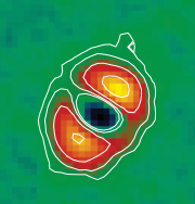
Herschel image of κ Coronae Borealis 31.1 parsecs away. This K giant is about twice as massive as our Sun. The red regions correspond to dust orbiting the star. Interestingly, this star also hosts at least one exoplanet with a mass of about 2 Jupiters. Credit: Bonsor et al. 2013.
Tutorial Video
If you’d like some quick tips about how to get started on Disk Detective, take a peek at this little video (below). I’m proud to say that this tutorial is the work of Disk Detective users, who wanted to help new users enjoy the site, and fill in some of the gaps in the other online instructions.
The concept for the video emerged from a round of discussion with Tadeáš Černohous, Phillip E. Griffith Sr., Doug Niergarth, Art Piipuu, Fernanda Piñeiro, John Reed, and Karl Wraight, Lily Lau and Hugo Durantini Luca. Lily Lau and Hugo Durantini Luca provided the footage and a draft of the script. I had the honor of narrating, and Scott Wiessenger, a video producer at NASA Goddard Space Flight Center, kindly edited it all together.
For official versions of the video in various formats, see this page at the Goddard Science Visualization Studio.
For more advance tips on how to use Disk Detective, you might enjoy these blog posts. And of course you can always contact us on the “Talk” network.
Best,
